Contextual Retrieval for Photo Albums: When Your 'Chunks' Are Pictures

Applying Anthropic’s Contextual Retrieval technique to personal photo libraries — where the notion of a “chunk” is a photo, not a paragraph.

---

Table of Contents

1. The Motivation
2. What Is Contextual Retrieval?
3. Contextual Chunks for Photos
4. System Design
5. Building the Contextual Description
6. Dual-Index Storage: ChromaDB + BM25
7. Hybrid Retrieval: Three Signals, One Ranking
8. CLIP: The Visual Signal
9. Answer Synthesis with a Local LLM
10. The Web UI
11. What I Learned
12. Key Takeaways

---

The Motivation

I was reading Anthropic’s Contextual Retrieval article while working on RAG-related projects at work, and one thing stuck with me: the core idea of enriching chunks with surrounding context before embedding them is simple, but the framing assumes your chunks are text. Paragraphs from a document. Sections from a manual.

But what if your chunks are photos?

I have thousands of photos sitting in folders on my Mac. When I want to find “that hiking trip near Portland in 2021,” I end up scrolling through months of thumbnails, squinting at timestamps, trying to remember which folder I put them in. Apple Photos and Google Photos solve this via ML (on-device, on-cloud, or hybrid), but I wanted something I could control and extend. Something that wouldn’t send my personal photos to a remote server.

That’s when the connection clicked: a photo is a chunk. And photos are rich with contextual information — EXIF metadata, GPS coordinates, visual content — that isn’t natively available to text-based RAG systems:

• EXIF metadata — Exchangeable Image File Format, a standard that embeds technical and contextual data directly into image files: timestamp, GPS coordinates, camera model, lens settings, and more
• GPS reverse geocoding — coordinates translated to “Portland, Oregon, United States”
• Filename hints — birthday_party.jpg tells you something IMG_4823.jpg doesn’t
• Visual content — what a vision model sees when it looks at the image

If I could assemble all of this into a single rich text description — a “contextual chunk” for a photo — then the entire Contextual Retrieval pipeline (semantic search + BM25 + reranking) could work on photos just as well as it works on documents.

That became this project: Photo Album RAG.

---

What Is Contextual Retrieval?

Before diving into the photo-specific design, it’s worth summarizing the technique from Anthropic’s original article.

Traditional RAG systems chunk documents into pieces, embed those pieces, and retrieve the most similar ones at query time. The problem is that chunking destroys context. A chunk saying “revenue grew 3%” is useless without knowing which company, which quarter, which filing. The embedding model only sees those four words.

Contextual Retrieval solves this by prepending context to each chunk before embedding. A language model reads the full document and generates a short summary for each chunk, explaining where it fits:

Original chunk:
  "The company's revenue grew by 3% over the previous quarter."

Contextualized chunk:
  "This chunk is from ACME Corp's Q2 2023 SEC filing; the previous
   quarter's revenue was $314M. The company's revenue grew by 3%
   over the previous quarter."

The contextualized chunk gets embedded, not the bare original. This gives the embedding model the information it needs to distinguish “ACME’s 3% growth” from “Beta Corp’s 3% growth.”

The article then shows that combining Contextual Embeddings (semantic search on enriched chunks) with Contextual BM25 (lexical search on enriched chunks) and reranking reduced retrieval failure rates by 67%. The key insight: semantic search and lexical search have complementary strengths. Semantic search understands meaning (“vacation” matches “holiday”), while BM25 catches exact keywords (“Portland” matches “Portland”). Fuse both, rerank, and you get a system that’s better than either alone.

This is the framework I adapted for photos.

---

Contextual Chunks for Photos

In a text document, context comes from surrounding paragraphs. In a photo, context comes from metadata and visual analysis. Here’s the mapping:

Text RAG	Photo RAG
Document	Photo library
Chunk	Single photo
Surrounding paragraphs	EXIF metadata + geocoding
LLM-generated context	Vision model caption
Contextualized chunk	Merged description (EXIF + location + caption)

A concrete example makes this clear. Consider a photo file IMG_2381.JPG. Without contextual enrichment, a search system sees a filename and raw pixels. With it:

Date taken: 2017:12:25 15:54:23.
Location: Los Angeles, California, United States.
Camera: Apple iPhone 6s.
Two people standing in front of a large decorated Christmas tree
on a sunny afternoon, palm trees visible in the background.
A busy outdoor shopping area with holiday decorations.

This text description is the contextual chunk. It gets embedded into a vector and also tokenized for BM25. Now a query like “Christmas in LA” matches on both semantic meaning and keywords. A query like “holiday photos with palm trees” matches on semantics even though the word “holiday” never appears in the chunk. And a query like “photos from December 2017” matches on the date string via BM25.

The richer the description, the better the retrieval. This is why caption quality matters more than anything else in this system.

---

System Design

The full pipeline looks like this:

INDEXING (run once, incremental)
──────────────────────────────────────────────────────────
Photo file
  -> Extract EXIF metadata      (date, GPS, camera)
  -> Reverse geocode GPS        (GPS -> "Portland, Oregon")
  -> Generate vision caption    (LLaVA via Ollama)
  -> Build contextual chunk     (EXIF + location + caption)
  -> Embed text                 (sentence-transformers)
  -> Store in ChromaDB          (vector index)
  -> Tokenize for BM25          (lexical index)
  -> [Optional] Embed pixels    (CLIP image embedding)

QUERYING (run any time)
──────────────────────────────────────────────────────────
Natural language query
  -> Stage 1a: Semantic search      (ChromaDB, top 50)
  -> Stage 1b: BM25 lexical search  (rank_bm25, top 50)
  -> Stage 1c: CLIP text->image     (optional, top 50)
  -> Stage 2:  Reciprocal Rank Fusion (merge + deduplicate)
  -> Stage 3:  Cross-encoder reranking (top 20 -> top K)
  -> Stage 4:  LLM answer synthesis   (Llama 3.2 via Ollama)

Everything runs locally. Ollama — a lightweight tool for running open-source LLMs locally on your machine — handles vision (LLaVA or Moondream) and text generation (Llama 3.2). It provides a simple API for pulling and serving models, with native support for Apple Silicon acceleration via Metal. ChromaDB provides persistent vector storage. BM25 handles keyword matching. The optional CLIP signal adds visual similarity search.

The project is structured as four modules:

src/photo_rag/
  ingest.py      # Indexing pipeline
  retrieve.py    # Hybrid retrieval + reranking
  clip_search.py # CLIP image embeddings (optional)
  query.py       # CLI + LLM answer synthesis
  app.py         # Streamlit web UI

---

Building the Contextual Description

The core of the indexing pipeline is the function that assembles the contextual chunk. Here’s the actual code from ingest.py:

def build_contextual_description(
    photo_path: Path,
    caption: str,
    meta: dict,
) -> str:
    """
    Combine EXIF metadata and vision caption into a single rich text
    description. This is the 'contextual chunk' from the Anthropic blog —
    it gives the embedding model rich, disambiguating context rather
    than bare pixels.
    """
    lines = []

    # Date
    if "datetime" in meta:
        lines.append(f"Date taken: {meta['datetime']}.")

    # Location
    if "gps" in meta:
        place = gps_to_place(*meta["gps"])
        if place:
            lines.append(f"Location: {place}.")
        else:
            lines.append(f"GPS coordinates: {meta['gps'][0]:.4f}, "
                         f"{meta['gps'][1]:.4f}.")

    # Camera
    if "camera" in meta:
        lines.append(f"Camera: {meta['camera']}.")

    # Filename (often has useful hints like "birthday" or "beach")
    stem = photo_path.stem.replace("_", " ").replace("-", " ")
    if not re.match(r"^(img|dsc|photo|p\d+)\s", stem, re.IGNORECASE):
        lines.append(f"Filename hint: {stem}.")

    # The actual visual description from the vision model
    if caption:
        lines.append(caption)

    return " ".join(lines)

A few design choices worth noting:

Filename filtering. Most phone photos are named IMG_xxxx or DSC_xxxx — those names carry zero information. The regex skips generic names and only includes filenames that might be meaningful (e.g., birthday_party.jpg becomes "Filename hint: birthday party.").

Reverse geocoding. Raw GPS coordinates like (45.5184, -122.7087) aren’t useful for text search. Nobody queries “photos at latitude 45.5.” The gps_to_place() function calls Nominatim (OpenStreetMap’s geocoder) to translate coordinates into “Portland, Oregon, United States” — now “photos from Portland” matches via both semantic search and BM25.

Vision captioning. The caption is generated by sending the photo to a local LLaVA model through Ollama:

def generate_caption(photo_path: Path) -> str:
    img = Image.open(photo_path).convert("RGB")
    img.thumbnail((1024, 1024), Image.LANCZOS)

    buf = io.BytesIO()
    img.save(buf, format="JPEG", quality=85)
    img_b64 = base64.b64encode(buf.getvalue()).decode()

    response = ollama.chat(
        model=VISION_MODEL,
        messages=[{
            "role": "user",
            "content": CAPTION_PROMPT,
            "images": [img_b64],
        }],
    )
    return response["message"]["content"].strip()

The prompt matters a lot here. The default focuses on concrete details:

Describe this photo in 2-3 sentences. Focus on: who or what is in it,
what activity or moment is happening, the setting or environment, and
the mood. Be specific. Do not say 'the image shows' — just describe
directly.

“Be specific” and “don’t say ‘the image shows’” are small prompt tweaks that meaningfully improve caption quality. Generic captions like “The image shows a beautiful outdoor scene” are nearly useless for retrieval. Specific captions like “Two people hiking on a forest trail with moss-covered trees and a wooden bridge over a stream” are information-dense and match a wide range of natural language queries.

---

Dual-Index Storage: ChromaDB + BM25

Each contextual description gets stored in two parallel indexes:

# Embed + store in ChromaDB (semantic search)
embedding = embedder.encode(description).tolist()
collection.add(
    ids=[photo_id],
    embeddings=[embedding],
    documents=[description],
    metadatas=[{
        "path": str(photo_path),
        "filename": photo_path.name,
        "datetime": meta.get("datetime", ""),
        "camera": meta.get("camera", ""),
        "caption": caption,
        "gps_lat": meta["gps"][0] if "gps" in meta else 0.0,
        "gps_lon": meta["gps"][1] if "gps" in meta else 0.0,
        "location": gps_to_place(*meta["gps"]) if "gps" in meta else "",
    }],
)

# Tokenize for BM25 (lexical search)
tokens = description.lower().split()
bm25_corpus.append(tokens)
bm25_ids.append(photo_id)

Why two indexes? Because semantic search and lexical search fail in different ways.

Semantic search (ChromaDB with all-MiniLM-L6-v2 embeddings) understands meaning. “Summer vacation” matches photos described as “sunny beach day” even without shared words. But it can struggle with specific proper nouns — “Portland” might not rank higher than “Seattle” if both appear in similar semantic contexts.

BM25 excels at exact keyword matching. “Portland” matches “Portland” with high confidence. “iPhone 6s” matches “iPhone 6s.” But it has no semantic understanding — “hiking” won’t match “trekking on a mountain trail.”

By running both and fusing the results, the system gets the best of both worlds. This is exactly the approach from the Contextual Retrieval article, and the results in that article showed a 49% reduction in retrieval failures when combining both signals versus using embeddings alone.

---

Hybrid Retrieval: Three Signals, One Ranking

At query time, the retriever runs a multi-stage pipeline:

def search(self, query: str, top_k: int = 5) -> list[PhotoResult]:
    # 1. Semantic search
    semantic_hits = self._semantic_search(query)

    # 2. BM25 search
    bm25_hits = self._bm25_search(query)

    # 3. CLIP search (if available)
    clip_hits = self._clip_search(query)

    # 4. Merge via RRF
    rrf_inputs = [semantic_hits, bm25_hits]
    if clip_hits:
        rrf_inputs.append(clip_hits)
    fused = self._reciprocal_rank_fusion(*rrf_inputs)

    # 5. Rerank the top pool
    pool = fused[:self.rerank_candidates]
    reranked = self._rerank(query, pool)

    return reranked[:top_k]

Reciprocal Rank Fusion (RRF)

The challenge with combining multiple retrieval signals is that their scores are on completely different scales. ChromaDB returns cosine similarities (0 to 1). BM25 returns TF-IDF-like scores (could be 0 to 50). CLIP returns cosine distances. You can’t average them without normalization, and normalization requires knowing the score distribution.

RRF sidesteps this problem by only using rank positions, not raw scores:

@staticmethod
def _reciprocal_rank_fusion(
    *result_lists: list[PhotoResult],
    k: int = 60,
) -> list[PhotoResult]:
    """
    RRF score = Sigma  1 / (k + rank_i)
    k=60 is the standard default.
    """
    rrf_scores: dict[str, float] = {}
    photo_by_id: dict[str, PhotoResult] = {}

    for result_list in result_lists:
        for rank, result in enumerate(result_list, start=1):
            pid = result.photo_id
            rrf_scores[pid] = rrf_scores.get(pid, 0.0) + 1.0 / (k + rank)
            photo_by_id[pid] = result

    fused = []
    for pid, score in sorted(rrf_scores.items(),
                             key=lambda x: x[1], reverse=True):
        photo = photo_by_id[pid]
        photo.rrf_score = score
        fused.append(photo)

    return fused

The formula 1 / (k + rank) gives diminishing credit for lower ranks, and k=60 dampens the influence of the very top positions.

Here’s a concrete example. Suppose you query “Christmas in LA” and get these top results from each signal:

Photo	Semantic Rank	BM25 Rank	RRF Score
IMG_2381 (Christmas tree, LA)	#1	#2	1/(60+1) + 1/(60+2) = 0.01639 + 0.01613 = 0.03252
IMG_0994 (holiday party)	#2	—	1/(60+2) = 0.01613
IMG_4412 (LA skyline)	#5	#1	1/(60+5) + 1/(60+1) = 0.01538 + 0.01639 = 0.03178
IMG_7721 (December sunset)	—	#3	1/(60+3) = 0.01587

IMG_2381 wins because it ranks highly in both signals — it’s the photo most consistently relevant across retrieval methods. IMG_4412 is #1 in BM25 (the keyword “LA” matches exactly) but only #5 in semantic search, so it scores slightly lower. IMG_0994 and IMG_7721 each appear in only one signal, so they drop to the bottom despite individually strong ranks.

The method is elegant because it requires no tuning and works regardless of how many signals you combine.

Cross-Encoder Reranking

After RRF produces a fused ranking, a cross-encoder (cross-encoder/ms-marco-MiniLM-L-6-v2) reranks the top candidates for final precision:

def _rerank(self, query: str, candidates: list[PhotoResult]) -> list[PhotoResult]:
    pairs = [(query, c.description) for c in candidates]
    scores = self.reranker.predict(pairs)

    for result, score in zip(candidates, scores):
        # Sigmoid normalization: raw logits -> 0-1 range
        result.rerank_score = 1.0 / (1.0 + math.exp(-float(score)))

    return sorted(candidates, key=lambda r: r.rerank_score, reverse=True)

Cross-encoders are fundamentally different from bi-encoders. A bi-encoder (like all-MiniLM-L6-v2) embeds the query and document separately, then compares vectors. A cross-encoder sees the query and document jointly — they’re concatenated and passed through the transformer together. This makes cross-encoders much more accurate at judging relevance, but too slow to run on the full index (hence why they’re used only on the top candidates after RRF narrows the field).

One practical detail: cross-encoders output raw logits, not probabilities. A score of -3 means “poor match” and +5 means “strong match,” but the scale is hard for users to interpret. We apply a sigmoid function to normalize scores to the 0-1 range, making them intuitive: 0.95 is a strong match, 0.3 is weak.

---

CLIP: The Visual Signal

The text-based pipeline (semantic + BM25) searches photos by their descriptions. CLIP adds a third signal that searches photos by their actual visual content.

CLIP (Contrastive Language-Image Pre-Training) encodes images and text into a shared embedding space. This means you can compare a text query directly to image pixels — “red sunset over ocean” can match a photo purely by what it looks like, even if the caption never mentioned sunsets or oceans.

During indexing, each photo is encoded into a CLIP vector and stored in a separate ChromaDB collection:

class CLIPIndexer:
    def add(self, photo_id: str, photo_path: Path):
        img = self.preprocess(Image.open(photo_path).convert("RGB"))
        img_tensor = img.unsqueeze(0).to(self.device)

        with self.torch.no_grad():
            embedding = self.model.encode_image(img_tensor)
            embedding = embedding / embedding.norm(dim=-1, keepdim=True)

        self.collection.add(
            ids=[photo_id],
            embeddings=[embedding.squeeze().cpu().tolist()],
            metadatas=[{"path": str(photo_path)}],
        )

At query time, the text query is encoded with CLIP’s text encoder and compared to all image embeddings. The results are fed into RRF alongside semantic and BM25 results — three signals fused into one ranking.

CLIP also enables something the text pipeline can’t do: image-to-image similarity search. Upload a photo, and the system finds visually similar photos in your library. This works by encoding the query image with the same CLIP model and comparing it to all stored image embeddings.

When Does CLIP Help?

CLIP is most valuable when:

• Captions are thin or missing. Some photos have no EXIF and get generic captions. CLIP can still match them by visual content.
• The query describes visual attributes. “Sunset,” “snow,” “crowded street” — these are visual concepts that CLIP handles well.
• You want “find photos like this one.” Image-to-image similarity is only possible with CLIP.

For a well-captioned library with rich EXIF data, the text pipeline alone is already strong. CLIP provides an incremental improvement on text queries but unlocks the entirely new capability of visual similarity search.

---

Answer Synthesis with a Local LLM

After retrieval returns the top-K photos, the system optionally generates a natural language answer using a local Llama 3.2 model through Ollama:

SYSTEM_PROMPT = """You are a helpful photo assistant. The user will ask
about their personal photo library. You will be given descriptions of the
most relevant photos retrieved for their query.

Your job is to:
1. Directly answer their question based on the photo descriptions.
2. Reference specific photos by filename and date.
3. If none of the photos match, say so honestly.
4. Keep your response concise and friendly.

Do not make up details that aren't in the descriptions."""


def answer_query(query: str, results: list[PhotoResult]) -> str:
    context = format_context(results)
    user_message = (
        f'The user asked: "{query}"\n\n'
        f"Here are the most relevant photos found:\n\n"
        f"{context}\n"
        f"Please answer the user's question based on these photos."
    )

    response = ollama.chat(
        model=ANSWER_MODEL,
        messages=[
            {"role": "system", "content": SYSTEM_PROMPT},
            {"role": "user", "content": user_message},
        ],
    )
    return response["message"]["content"].strip()

The LLM sees the contextual descriptions — the same enriched text that was used for indexing — and synthesizes a human-readable answer. For example, querying “photos from my trip to Japan” might return:

I found 2 photos from Japan! IMG_1629.JPG was taken on June 6, 2017 in Kyoto — it shows a traditional temple entrance with wooden gates and stone lanterns. IMG_1633.JPG from the same day shows a bamboo grove path with dappled sunlight filtering through the tall stalks.

This is the “generation” in Retrieval-Augmented Generation — the LLM doesn’t hallucinate about photos it hasn’t seen, because the system prompt explicitly constrains it to the retrieved descriptions.

---

The Web UI

The project includes a Streamlit web UI that brings everything together in a browser:

uv run photo-app
# Opens at http://localhost:8501

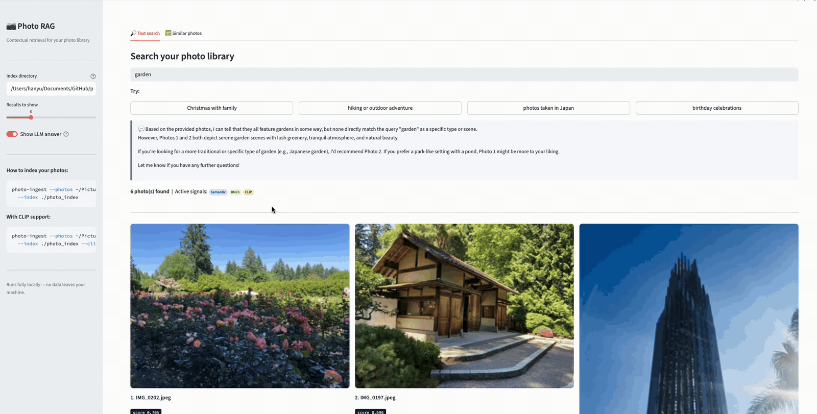
Here’s a short demo of the app in action. In this example, the user searches for “garden” — and the results show how hybrid retrieval pulls photos from multiple signals. Some photos match because the vision model caption describes a garden scene (semantic match via visual content). Others match because their reverse-geocoded location includes “Garden Grove” (lexical match via BM25). This is exactly the kind of complementary retrieval that the hybrid approach enables — neither signal alone would have surfaced all of these results:

Searching “garden” in Photo Album RAG — results include both visually recognized gardens and photos geotagged in Garden Grove, demonstrating hybrid retrieval across semantic and lexical signals.

Now watch what happens when we augment the query to “garden from portland.” The added location keyword gives BM25 a strong lexical signal — “Portland” matches the reverse-geocoded location in the contextual descriptions. As a result, actual garden photos from Portland rise to the top, while the Garden Grove photos (which matched “garden” lexically but not “Portland”) drop in rank. This is the benefit of the dual-indexing strategy: by combining semantic understanding with keyword precision, users can progressively refine their queries to get more accurate results.

Searching “garden from portland” — adding a location keyword sharpens the results, pushing Portland garden photos to the top while Garden Grove photos drop in rank.

The UI provides two modes:

Text search — Type a natural language query, see a thumbnail grid of matching photos with metadata (date, camera, location) and relevance scores, plus an optional LLM-generated answer.

Visual similarity — Upload or select a photo, find visually similar photos via CLIP. Each result card includes a “Find similar” button for iterative visual exploration.

One practical detail worth mentioning: iPhone photos often have an EXIF orientation tag — the pixels are stored rotated, with metadata indicating how to display them correctly. Without handling this, photos appear sideways in the UI. A one-line fix using Pillow’s ImageOps.exif_transpose() corrects this:

def load_thumbnail(path: str, size: int = 300) -> Image.Image | None:
    try:
        img = Image.open(path)
        img = ImageOps.exif_transpose(img)  # fix orientation
        img.thumbnail((size, size), Image.LANCZOS)
        return img
    except Exception:
        return None

Small details like this matter a lot for usability — a search system that returns the right photos but displays them sideways feels broken.

---

What I Learned

Caption Quality Dominates Everything

The single biggest lever for retrieval quality is the vision model caption. A specific, detailed caption makes the photo findable by a wide range of queries. A generic caption makes it nearly invisible.

The prompt I landed on — asking the model to focus on who, what, where, and mood, while avoiding filler phrases like “the image shows” — was the result of iteration. Small prompt changes had outsized effects on retrieval quality.

EXIF Is Underrated

I expected the vision caption to do most of the heavy lifting. In practice, EXIF metadata — especially reverse-geocoded locations and timestamps — contributed as much or more to retrieval quality for many query types. “Photos from Portland” works because of GPS geocoding, not because LLaVA mentioned Portland. “Photos from December 2017” works because of EXIF timestamps.

The lesson: don’t overlook structured metadata when building RAG systems. It’s free context that costs nothing to extract and dramatically improves recall for factual queries.

BM25 Earns Its Keep

It would be tempting to skip BM25 and just use semantic search — it’s simpler, one less index to maintain. But BM25 consistently caught results that semantic search missed, particularly for:

• Specific place names (“Kyoto”, “Portland”)
• Camera models (“iPhone 6s”)
• Exact date strings (“2017:12:25”)

These are exact keyword matches where BM25’s term-frequency scoring outperforms embedding similarity. The hybrid approach is worth the added complexity.

Sigmoid-Normalized Scores Are More Useful

Cross-encoder models output raw logits, which can be any real number. A score of -2.3 or +4.7 is meaningless to a user. Applying a sigmoid function to map scores to the 0-1 range makes them immediately interpretable: 0.92 is clearly a strong match, 0.15 is clearly weak. This is a small change that significantly improves the user experience.

Everything Local Is a Feature

Running the entire pipeline locally — Ollama for vision and text generation, ChromaDB for storage, sentence-transformers for embeddings — means no photos leave your machine. For a personal photo library, this isn’t just a nice-to-have; it’s the only acceptable architecture for many people. The tradeoff is speed: LLaVA captioning is the bottleneck during indexing, especially on CPU. On Apple Silicon with Metal acceleration, it’s reasonable.

---

Key Takeaways

1. Contextual Retrieval generalizes beyond text. The Anthropic article frames contextual chunking in terms of documents and paragraphs. But the core principle — enrich your chunks with surrounding context before embedding — applies to any domain where chunks lack sufficient standalone information. Photos are a natural fit.

2. The “contextual chunk” for a photo is its combined metadata + caption. EXIF metadata (date, GPS, camera), reverse-geocoded location, filename hints, and a vision model caption together form a rich text description that makes the photo searchable by natural language.

3. Hybrid retrieval (semantic + BM25 + CLIP) outperforms any single signal. Semantic search understands meaning. BM25 catches exact keywords. CLIP matches visual content. Reciprocal Rank Fusion combines them without needing to normalize incompatible score scales.

4. Cross-encoder reranking is the precision layer. Bi-encoders are fast but approximate. Cross-encoders are slow but accurate. Using cross-encoders to rerank a small candidate pool (after RRF narrows the field) gives you the best of both.

5. Caption quality is the single biggest lever. A specific, detailed vision model caption makes a photo findable by dozens of query variations. A generic caption makes it nearly invisible. Invest time in your captioning prompt.

6. Fully local AI is practical today. Ollama + ChromaDB + sentence-transformers + open-clip — the entire stack runs on a laptop. Apple Silicon with Metal makes it fast enough for personal use. No cloud, no API keys, no data leaving your machine.

---

The full project is on GitHub: bearbearyu1223/photo-album-rag

All opinions expressed are my own.