Study Notes: Stanford CS336 Language Modeling from Scratch [13]

Fine-Tuning Qwen3-1.7B on Lambda Labs for Math Reasoning

When developing machine learning training pipelines, there’s often a disconnect between local development environments and production-scale cloud infrastructure. You might prototype on your laptop (say, a MacBook with Apple Silicon), only to discover that your code breaks on CUDA GPUs, or that patterns that worked locally don’t scale in the cloud.

In this post, I’ll share my workflow for developing Supervised Fine-Tuning (SFT) code on a MacBook with Apple Silicon, testing it locally, then seamlessly deploying to cloud instances like Lambda Labs.

This workflow was developed while implementing SFT for Qwen3-1.7B on the MATH dataset, but the principles apply broadly to any PyTorch-based training pipeline development.

All code is available on GitHub: bearbearyu1223/qwen3_supervised_fine_tuning

Table of Contents

• Fine-Tuning Qwen3-1.7B on Lambda Labs for Math Reasoning
  • Table of Contents
  • The Challenge: Bridging Local and Cloud Development
  • Part 1: Setting Up Local Development Environment
    • Why Apple Silicon for ML Development?
    • Why Qwen3-1.7B as the Base Model?
    • Project Structure and Package Management
  • Part 2: Writing Device-Agnostic Training Code
    • Automatic Hardware Detection
    • Numerical Precision Considerations
    • Gradient Accumulation for Memory Efficiency
  • Part 3: The Training Pipeline
    • Data Preparation: The MATH Dataset
    • The r1_zero Prompt Format
    • Response Masking for SFT
  • Part 4: Local Testing and Validation
    • Quick Sanity Checks
    • Inference Backend: Local vs Cloud
  • Part 5: Scaling with HuggingFace Accelerate
    • Why HuggingFace Accelerate
    • Code Changes for Multi-GPU Support
  • Part 6: Deploying to Lambda Cloud
    • Step-by-Step Deployment
  • Part 7: Evaluation Pipeline
    • Math Answer Grading
    • Running Evaluation
    • Results: Before and After SFT
  • Part 8: Practical Recommendations
    • Development Workflow Summary

The Challenge: Bridging Local and Cloud Development

My typical ML development workflow faces a fundamental tension—I use a MacBook Pro with M-series chips for personal side projects, which creates some tradeoffs:

Environment	Pros	Cons
Local (MacBook)	Fast iteration, no cost, familiar tools	Limited memory, slower training, no CUDA
Cloud (Lambda)	Powerful GPUs, scalable, CUDA support	Setup overhead, costs money, less interactive

The ideal workflow would let me:

1. Develop locally with fast feedback loops
2. Test easily before committing cloud resources
3. Deploy seamlessly without rewriting code
4. Scale horizontally when more compute is available

This post presents a battle-tested approach to achieving all four.

Part 1: Setting Up Local Development Environment

Why Apple Silicon for ML Development?

Beyond personal preference, Apple Silicon Macs offer a genuinely compelling development environment:

• Unified Memory Architecture: 16–64GB RAM shared between CPU and GPU
• Metal Performance Shaders (MPS): PyTorch backend for GPU acceleration
• Power Efficiency: Extended battery life for portable development
• Native ARM: Fast Python and native tool execution

However, there are important limitations:

Feature	CUDA (NVIDIA)	MPS (Apple Silicon)
Float16 Training	Stable with gradient scaling	Often causes NaN losses
BFloat16	Full support (Ampere+)	Limited support
Multi-GPU	NCCL, NVLink	Single GPU only
Flash Attention	Available	Not available
Memory	Dedicated VRAM	Shared system RAM

Key Insight: MPS (Metal Performance Shaders—Apple’s GPU-accelerated compute framework) is excellent for development and testing but usually requires float32 precision for numerical stability.

Why Qwen3-1.7B as the Base Model?

Choosing the right base model is critical for SFT projects. I selected Qwen3-1.7B for several reasons:

1. Right-sized for the task

Model Size	Local Dev (32GB Mac)	Single A100 (40GB)	Training Time
0.5B–1B	Comfortable	Very fast	Minutes
1.7B	Workable	Fast	~1 hour
4B–8B	Challenging	Comfortable	Hours
14B+	Not feasible	Tight fit	Many hours

At 1.7B parameters, Qwen3-1.7B hits a sweet spot: small enough to iterate quickly on a MacBook during development, yet large enough to demonstrate meaningful learning on complex math problems.

2. Strong base capabilities

Qwen3 models come with several architectural improvements:

• Improved tokenizer: Better handling of mathematical notation and LaTeX
• Extended context: 32K context window for longer reasoning chains
• Thinking mode support: Native support for <think> tags that align with our r1_zero format

3. Active ecosystem

• Regular updates from Alibaba’s Qwen team
• Good HuggingFace Transformers integration
• Compatible with vLLM for fast inference
• Apache 2.0 license for commercial use

4. Qwen3 model family options

The Qwen3 family provides a natural scaling path:

Model	Parameters	Use Case
Qwen3-0.6B	0.6B	Rapid prototyping, edge deployment
Qwen3-1.7B	1.7B	Development, single-GPU training
Qwen3-4B	4B	Production fine-tuning
Qwen3-8B	8B	High-quality results, multi-GPU
Qwen3-14B/32B	14B/32B	State-of-the-art, distributed training

Starting with 1.7B allows rapid iteration. Once the pipeline is validated, scaling up to 4B or 8B for better results is straightforward—the same code works across all sizes.

Project Structure and Package Management

I use uv for fast, reproducible Python package management.

Install uv:

curl -LsSf https://astral.sh/uv/install.sh | sh

Project structure:

qwen3_supervised_fine_tuning/
├── cs336_alignment/
│   ├── __init__.py
│   ├── sft.py              # Main training code
│   ├── evaluate_math.py    # Evaluation utilities
│   ├── drgrpo_grader.py    # Math grading functions
│   └── prompts/
│       └── r1_zero.prompt  # Prompt template
├── scripts/
│   ├── run_sft.py          # Training entry point
│   ├── run_math_eval.py    # Evaluation entry point
│   ├── download_model.py   # Model downloader
│   └── download_math.py    # Data downloader
├── data/math/              # MATH dataset
├── pyproject.toml          # Dependencies
└── uv.lock                 # Locked versions

pyproject.toml with optional CUDA dependencies:

[project]
name = "qwen3-sft"
requires-python = ">=3.11,<3.13"
dependencies = [
    "accelerate>=1.5.2",
    "torch",
    "transformers>=4.50.0",
    "datasets>=3.0.0",
    "tqdm>=4.67.1",
    "matplotlib>=3.8.0",
]

[project.optional-dependencies]
cuda = [
    "flash-attn==2.7.4.post1",
]

Local installation:

uv sync              # Basic install (Mac/CPU)
uv sync --extra cuda # With CUDA extras (Linux with GPU)

Part 2: Writing Device-Agnostic Training Code

The key to seamless local-to-cloud transitions is writing code that adapts to available hardware without manual changes.

Automatic Hardware Detection

The training code implements sophisticated automatic device detection:

def detect_compute_environment(model_name_or_path: str) -> ComputeEnvironment:
    """Detect hardware and recommend optimal training settings."""

    if torch.cuda.is_available():
        num_gpus = torch.cuda.device_count()
        device_name = torch.cuda.get_device_name(0)
        total_memory_gb = torch.cuda.get_device_properties(0).total_memory / (1024**3)
        supports_bf16 = torch.cuda.is_bf16_supported()
        return ComputeEnvironment(
            device="cuda",
            num_gpus=num_gpus,
            memory_gb=total_memory_gb,
            supports_bf16=supports_bf16,
            ...
        )

    elif torch.backends.mps.is_available():
        # Extract memory via sysctl on macOS
        memory_gb = get_mac_memory()
        return ComputeEnvironment(
            device="mps",
            num_gpus=1,
            memory_gb=memory_gb,
            supports_bf16=False,  # MPS has limited BF16 support
            ...
        )

    else:
        return ComputeEnvironment(device="cpu", ...)

This allows running with --auto to automatically detect and configure optimal settings:

uv run scripts/run_sft.py --auto \
    --model-name-or-path models/qwen3-1.7b \
    --train-data-path data/math/train.jsonl \
    --output-dir outputs/sft_qwen3

Numerical Precision Considerations

This is where many developers encounter their first “works locally, fails on cloud” (or vice versa) bug:

def get_dtype_and_precision(device: str) -> tuple[torch.dtype, str]:
    """
    Determine appropriate dtype and mixed precision setting.

    Critical insight: MPS does NOT support float16 training reliably.
    Using float16 on MPS often results in NaN losses.
    """
    if device == "cuda":
        # CUDA: Use bfloat16 if available (Ampere+), else float16
        if torch.cuda.is_bf16_supported():
            return torch.bfloat16, "bf16"
        else:
            return torch.float16, "fp16"
    else:
        # MPS and CPU: Use float32 for numerical stability
        return torch.float32, "no"

Why This Matters:

Device	Recommended Dtype	Reason
CUDA (Ampere+)	bfloat16	Best balance of speed and stability
CUDA (older)	float16	With gradient scaling
MPS	float32	float16 causes NaN losses
CPU	float32	No mixed precision benefit

Gradient Accumulation for Memory Efficiency

With limited memory on laptops, gradient accumulation is essential. The code computes optimal settings based on available hardware:

# Memory estimation (rough heuristics)
if device == "cuda":
    memory_per_batch = model_size_billions * 6  # fp16 training
elif device == "mps":
    memory_per_batch = model_size_billions * 12  # fp32 + shared memory
else:
    memory_per_batch = model_size_billions * 16

# Compute max batch size with 70% safety margin
max_batch_size = int((available_memory_gb * 0.7) / memory_per_batch)
max_batch_size = max(1, min(max_batch_size, device_caps[device]))

# Compute gradient accumulation for target effective batch
gradient_accumulation_steps = max(1, target_effective_batch // max_batch_size)

Memory Scaling Recommendations for Qwen3-1.7B:

Device	Memory	batch_size	gradient_accumulation_steps	Effective Batch
MacBook M-series	16–32GB	1–2	8–16	16
NVIDIA A100 (40GB)	40GB	8	2	16
NVIDIA A100 (80GB)	80GB	16	1	16

Part 3: The Training Pipeline

Data Preparation: The MATH Dataset

The MATH dataset is a collection of 12,500 challenging competition mathematics problems (12,000 train / 500 test). Each problem includes a detailed step-by-step solution, making it ideal for training models on mathematical reasoning.

Dataset Structure:

Each example contains:

• problem: The math question
• solution: Step-by-step solution with reasoning
• answer: Final answer (often in \boxed{} format)
• subject: One of 7 mathematical topics
• level: Difficulty from 1 (easiest) to 5 (hardest)

Subject Distribution:

The dataset covers 7 mathematical topics:

Subject	Description
Prealgebra	Basic arithmetic, fractions, percentages
Algebra	Equations, polynomials, functions
Number Theory	Divisibility, primes, modular arithmetic
Counting & Probability	Combinatorics, probability theory
Geometry	Triangles, circles, coordinate geometry
Intermediate Algebra	Complex equations, series, inequalities
Precalculus	Trigonometry, vectors, complex numbers

Example Problems by Difficulty:

Here are examples showing the range of difficulty levels:

---

Level 2 (Prealgebra) — Straightforward algebraic manipulation:

Problem: If $5x - 3 = 12$, what is the value of $5x + 3$?

Solution: Adding 6 to both sides of $5x - 3 = 12$ gives $5x - 3 + 6 = 12 + 6$. Simplifying both sides gives $5x + 3 = \boxed{18}$.

Answer: 18

---

Level 3 (Algebra) — Requires understanding of functions:

Problem: How many vertical asymptotes does the graph of $y=\frac{2}{x^2+x-6}$ have?

Solution: The denominator of the rational function factors into $x^2+x-6=(x-2)(x+3)$. Since the numerator is always nonzero, there is a vertical asymptote whenever the denominator is $0$, which occurs for $x = 2$ and $x = -3$. Therefore, the graph has $\boxed{2}$ vertical asymptotes.

Answer: 2

---

Level 4 (Geometry) — Multi-step geometric reasoning:

Problem: In triangle $\triangle ABC$, we have that $AB = AC = 14$ and $BC = 26$. What is the length of the shortest angle bisector in $ABC$? Express your answer in simplest radical form.

Solution: The shortest angle bisector will be from vertex $A$. Since $\triangle ABC$ is isosceles, the angle bisector from $A$ is also the perpendicular bisector of $BC$. Using the Pythagorean theorem with $AC = 14$ and $DC = \frac{1}{2} \cdot BC = 13$, we find $AD^2 = AC^2 - CD^2 = 14^2 - 13^2 = 27$. Therefore, $AD = \boxed{3\sqrt{3}}$.

Answer: 3\sqrt{3}

---

Level 5 (Counting & Probability) — Complex multi-case reasoning:

Problem: Ryan has 3 red lava lamps and 3 blue lava lamps. He arranges them in a row on a shelf randomly, then turns 3 random lamps on. What is the probability that the leftmost lamp on the shelf is red, and the leftmost lamp which is turned on is also red?

Solution: There are $\binom{6}{3}=20$ ways to arrange the lamps, and $\binom{6}{3}=20$ ways to choose which are on, giving $20 \cdot 20=400$ total outcomes. Case 1: If the left lamp is on, there are $\binom{5}{2}=10$ ways to choose other on-lamps and $\binom{5}{2}=10$ ways to choose other red lamps, giving 100 possibilities. Case 2: If the left lamp isn’t on, there are $\binom{5}{3}=10$ ways to choose on-lamps, and $\binom{4}{1}=4$ ways to choose the other red lamp, giving 40 possibilities. Total: $\frac{140}{400}=\boxed{\frac{7}{20}}$.

Answer: \dfrac{7}{20}

---

Download the dataset:

uv run python scripts/download_math.py

The r1_zero Prompt Format

The training uses the r1_zero prompt format which encourages chain-of-thought reasoning:

A conversation between User and Assistant. The User asks a question,
and the Assistant solves it. The Assistant first thinks about the
reasoning process in the mind and then provides the User with the answer.
The reasoning process is enclosed within <think> </think> and answer
is enclosed within <answer> </answer> tags, respectively.

User: {question}
Assistant: <think>
{reasoning}
</think> <answer> {answer} </answer>

This format teaches the model to:

1. Think through the problem step-by-step in <think> tags
2. Provide a clear final answer in <answer> tags

Response Masking for SFT

A key implementation detail: we only compute loss on response tokens, not the prompt:

class MathSFTDataset(Dataset):
    def __getitem__(self, idx):
        # Tokenize prompt and response separately
        prompt_tokens = self.tokenizer(prompt, ...)
        response_tokens = self.tokenizer(response, ...)

        # Create response mask: 1 for response, 0 for prompt/padding
        response_mask = torch.cat([
            torch.zeros(len(prompt_tokens)),
            torch.ones(len(response_tokens)),
            torch.zeros(padding_length)
        ])

        return {
            "input_ids": input_ids,
            "attention_mask": attention_mask,
            "response_mask": response_mask,
        }

The loss is then computed only on response tokens:

# NLL loss normalized by response tokens
nll_loss = masked_normalize(
    tensor=-policy_log_probs,
    mask=response_mask,
    normalize_constant=num_response_tokens,
)

Part 4: Local Testing and Validation

Before deploying to cloud, thorough local testing saves time and money.

Quick Sanity Checks

# Test with minimal samples to verify pipeline works
uv run python scripts/run_sft.py \
    --model-name-or-path models/qwen3-1.7b \
    --train-data-path data/math/train.jsonl \
    --output-dir outputs/sft_test \
    --num-samples 10 \
    --num-epochs 1 \
    --batch-size 1 \
    --gradient-accumulation-steps 2

What to verify:

1. Model loads without errors
2. Data pipeline produces valid batches
3. Loss decreases (not NaN or constant)
4. Checkpoints save correctly
5. Model can be reloaded from checkpoint

Inference Backend: Local vs Cloud

A key challenge when developing on Apple Silicon is that vLLM—the go-to inference engine for fast LLM serving—requires CUDA and doesn’t run on Macs. The evaluation code handles this with two backends:

Environment	Inference Backend	Why
Local (MPS)	HuggingFace Transformers	Pure PyTorch, runs anywhere
Cloud (CUDA)	vLLM	Optimized kernels, 10–20× faster

def get_inference_backend(model_path: str, device: str):
    """Return appropriate inference backend for the current environment."""
    if device == "cuda" and is_vllm_available():
        from vllm import LLM
        return VLLMBackend(LLM(model=model_path))
    else:
        # Fallback to HuggingFace for MPS/CPU
        from transformers import AutoModelForCausalLM, AutoTokenizer
        model = AutoModelForCausalLM.from_pretrained(model_path).to(device)
        tokenizer = AutoTokenizer.from_pretrained(model_path)
        return TransformersBackend(model, tokenizer)

Part 5: Scaling with HuggingFace Accelerate

Why HuggingFace Accelerate

Feature	Manual DDP	Accelerate
Code changes	Significant	Minimal
Device placement	Manual	Automatic
Gradient sync	Manual	Automatic
Mixed precision	Manual setup	One flag
Single/Multi GPU	Different code paths	Same code

Code Changes for Multi-GPU Support

The key changes to support multi-GPU:

from accelerate import Accelerator

def train_sft(config):
    # Initialize Accelerator
    accelerator = Accelerator(
        gradient_accumulation_steps=config.gradient_accumulation_steps,
        mixed_precision="bf16" if device == "cuda" else "no",
    )

    # Prepare model, optimizer, dataloader
    model, optimizer, dataloader, scheduler = accelerator.prepare(
        model, optimizer, dataloader, scheduler
    )

    for batch in dataloader:
        # Use accelerator's gradient accumulation context
        with accelerator.accumulate(model):
            loss = compute_loss(model, batch)
            accelerator.backward(loss)

            if accelerator.sync_gradients:
                accelerator.clip_grad_norm_(model.parameters(), max_norm)

            optimizer.step()
            scheduler.step()
            optimizer.zero_grad()

    # Save only on main process
    if accelerator.is_main_process:
        unwrapped_model = accelerator.unwrap_model(model)
        unwrapped_model.save_pretrained(output_dir)

Key Accelerate Patterns:

1. accelerator.prepare(): Wraps objects for distributed training
2. accelerator.accumulate(): Handles gradient accumulation correctly
3. accelerator.backward(): Syncs gradients across devices
4. accelerator.sync_gradients: True when accumulation cycle completes
5. accelerator.is_main_process: Only one process logs/saves

Part 6: Deploying to Lambda Cloud

Step-by-Step Deployment

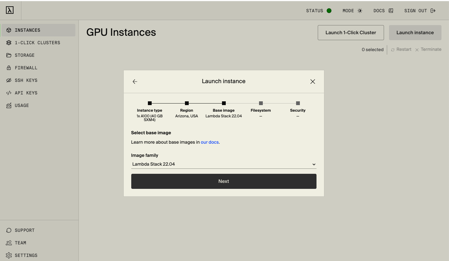
This guide uses a 1x A100 40GB SXM4 instance on Lambda Cloud.

Step 1: Launch Instance and SSH

Go to Lambda Cloud and launch a 1x A100 40GB SXM4 instance

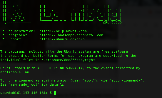
SSH into your instance:

ssh ubuntu@<your-instance-ip>

Step 2: Clone and Setup Environment

# Clone the repository
git clone https://github.com/bearbearyu1223/qwen3_supervised_fine_tuning.git
cd qwen3_supervised_fine_tuning

# Install uv package manager
curl -LsSf https://astral.sh/uv/install.sh | sh

# Install dependencies 
uv sync 

# Install dependecies with CUDA support for flash-attn and vLLM
uv sync --extra cuda

Step 3: Download Model and Data

uv run python scripts/download_model.py --model-name Qwen/Qwen3-1.7B
uv run python scripts/download_math.py

Step 4: Run SFT Training

# Run with AUTO mode (auto-detects GPU and optimal settings)
uv run accelerate launch scripts/run_sft.py --auto \
    --model-name-or-path models/qwen3-1.7b \
    --train-data-path data/math/train.jsonl \
    --output-dir outputs/sft_qwen3

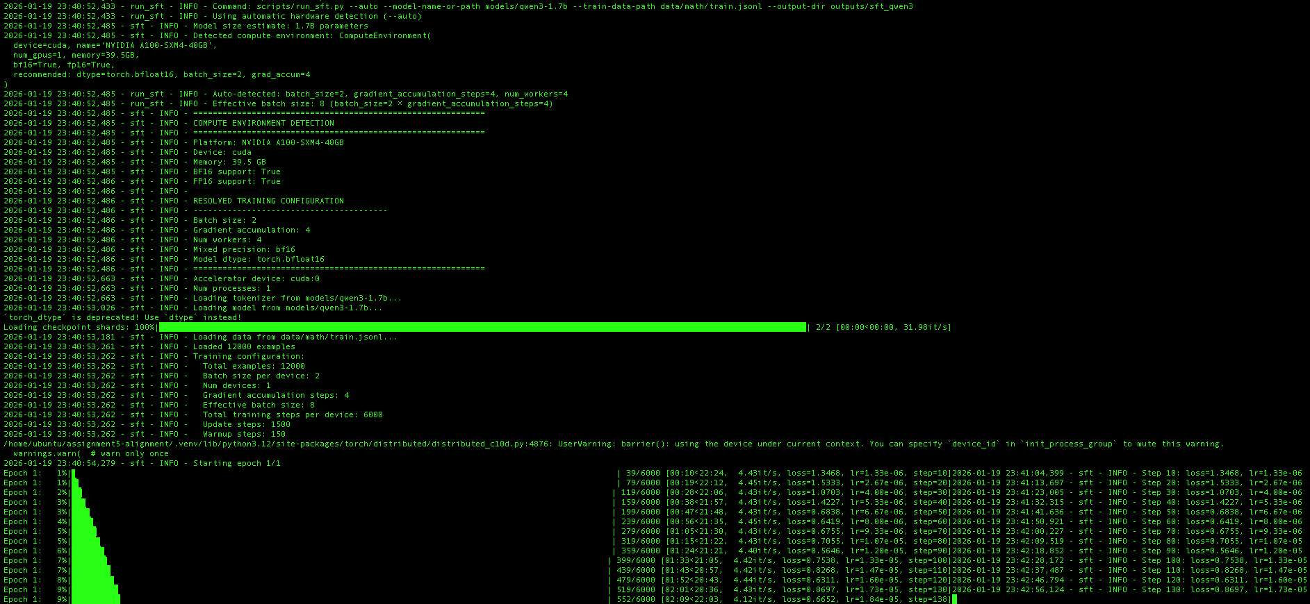
The --auto flag triggers automatic compute environment detection. On this Lambda instance, the script detected:

Setting	Value
Platform	NVIDIA A100-SXM4-40GB
Device	cuda
Memory	39.5 GB
BF16 Support	True
FP16 Support	True

Based on these capabilities, the training configuration was automatically resolved to:

Parameter	Auto-Selected Value
Batch size	2
Gradient accumulation	4
Effective batch size	8
Mixed precision	bf16
Model dtype	torch.bfloat16
Num workers	4

The training then proceeds through 12,000 examples (the full MATH training set) for 1,500 update steps. The training curves below show the loss and learning rate schedule:

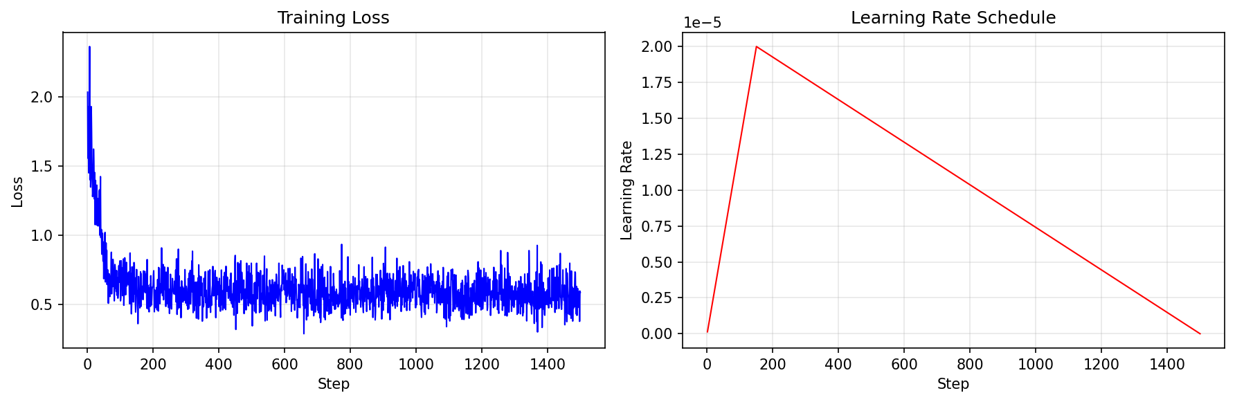
The left plot shows the training loss dropping rapidly from ~2.3 to ~0.7 in the first 100 steps, then gradually decreasing to ~0.5 by the end of training. The right plot shows the learning rate schedule: a linear warmup to 2e-5 followed by linear decay to zero.

Step 5: Evaluate the Trained Model

uv run python scripts/run_math_eval.py \
    --model-name-or-path outputs/sft_qwen3/final \
    --output-path outputs/sft_qwen3_eval.jsonl

Part 7: Evaluation Pipeline

Math Answer Grading

The evaluation uses a sophisticated grading pipeline that handles the complexity of mathematical answers:

def r1_zero_reward_fn(response: str, ground_truth: str) -> dict:
    """
    Grade a model response against the ground truth.

    Returns:
        format_reward: 1.0 if response has correct <think>/<answer> format
        answer_reward: 1.0 if answer is mathematically correct
        reward: Combined reward
    """
    # Check format: must have "</think> <answer>" and "</answer>" tags
    if "</think> <answer>" not in response or "</answer>" not in response:
        return {"format_reward": 0.0, "answer_reward": 0.0, "reward": 0.0}

    # Extract answer from tags
    model_answer = response.split("<answer>")[-1].replace("</answer>", "")

    # Handle \boxed{} format
    if "\\boxed" in model_answer:
        model_answer = extract_boxed_answer(model_answer)

    # Grade using multiple strategies
    is_correct = grade_answer(model_answer, ground_truth)

    return {
        "format_reward": 1.0,
        "answer_reward": 1.0 if is_correct else 0.0,
        "reward": 1.0 if is_correct else 0.5,  # Partial credit for format
    }

The grading uses multiple strategies with timeout protection:

1. MATHD normalization: Dan Hendrycks’ string normalization
2. Sympy symbolic equality: For algebraic equivalence
3. math_verify library: Advanced parsing for complex expressions

Running Evaluation

Zero-shot evaluation (baseline):

uv run python scripts/run_math_eval.py \
    --model-name-or-path models/qwen3-1.7b \
    --output-path outputs/qwen3_base_eval.jsonl

Fine-tuned model evaluation:

uv run python scripts/run_math_eval.py \
    --model-name-or-path outputs/sft_qwen3/final \
    --output-path outputs/sft_qwen3_eval.jsonl

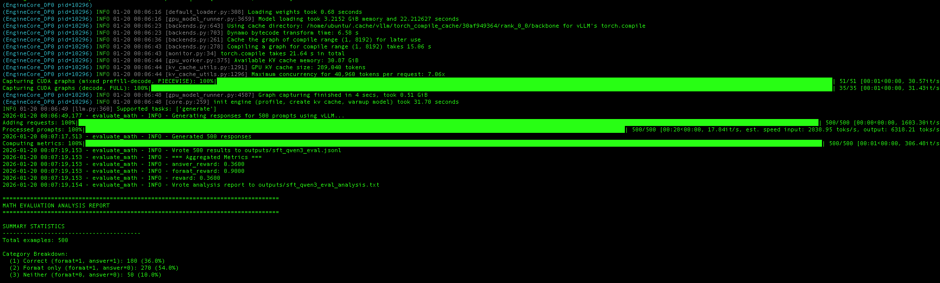
On CUDA, the evaluation script automatically uses vLLM for high-throughput inference. The screenshot shows vLLM’s initialization process:

1. Model loading: The fine-tuned model loads into ~3.2 GB of GPU memory
2. CUDA graph compilation: vLLM compiles optimized CUDA graphs for the decode phase
3. KV cache allocation: With 30.87 GB available, vLLM allocates a KV cache supporting ~209K tokens

Once initialized, vLLM generates responses for all 500 test problems at impressive speeds—approximately 17,800 tokens/second throughput, with input processing at ~2,800 toks/s and output generation at ~6,300 toks/s. The entire evaluation completes in under 30 seconds, compared to several minutes with standard HuggingFace inference.

The aggregated metrics show the final results: 36% answer accuracy (answer_reward: 0.36) and 90% format compliance (format_reward: 0.90).

Results: Before and After SFT

After training Qwen3-1.7B on ~12K examples from the MATH dataset with only one epoch, here are the evaluation results on 500 test problems:

Metric	Base Model (Zero-Shot)	After SFT	Improvement
Correct Answers	133 (26.6%)	180 (36.0%)	+9.4pp (+35% relative)
Format Compliance	148 (29.6%)	450 (90.0%)	+60.4pp (+204% relative)
Format Only (wrong answer)	15 (3.0%)	270 (54.0%)	—
Neither (no format, wrong)	352 (70.4%)	50 (10.0%)	-60.4pp

Key Observations:

1. Dramatic format improvement: The base Qwen3-1.7B model doesn’t naturally output the <think>...</think> <answer>...</answer> format. After SFT, 90% of responses follow the expected format—a critical requirement for downstream applications that parse structured outputs.

2. Meaningful accuracy gains: Correct answers improved from 26.6% to 36.0%, a 35% relative improvement. While there’s still room for growth, this demonstrates the model is learning genuine mathematical reasoning, not just format mimicry.

3. The “format only” category: After SFT, 54% of responses have correct format but wrong answers. These are cases where the model follows the reasoning structure but makes mathematical errors—a good target for future improvements like RLHF or more training data.

Example: Before SFT (Base Model)

The base model often ignores the expected format entirely:

Problem: What is the smallest positive perfect cube that can be written
         as the sum of three consecutive integers?

Base Model Output:
</think>
</think>
To solve this problem, we need to find the smallest positive perfect cube
that can be expressed as the sum of three consecutive integers.
Let the three consecutive integers be $ n-1 $, $ n $, and $ n+1 $.
The sum of these three integers is: $(n-1) + n + (n+1) = 3n$
...

Notice the malformed </think></think> without opening tags or <answer> tags.

Example: After SFT

The fine-tuned model produces well-structured reasoning:

Problem: What is the smallest positive perfect cube that can be written
         as the sum of three consecutive integers?

SFT Model Output:
Let the three consecutive integers be $n-1$, $n$, and $n+1$. Then
$(n-1)+n+(n+1)=3n$. We want to find the smallest positive perfect cube
that is divisible by 3. The smallest positive perfect cube divisible
by 3 is $3^3=27$. Therefore, the smallest positive perfect cube that
can be written as the sum of three consecutive integers is $\boxed{27}$.
</think> <answer>\boxed{27}</answer>

The SFT model shows clear reasoning followed by a properly formatted answer.

Part 8: Practical Recommendations

Development Workflow Summary

+------------------------------------------------------------------+
|                    LOCAL DEVELOPMENT (Mac)                       |
+------------------------------------------------------------------+
|  1. Write code with device-agnostic patterns                     |
|  2. Test with small samples (--num-samples 10)                   |
|  3. Verify loss decreases, no NaN                                |
|  4. Commit and push to GitHub                                    |
+------------------------------------------------------------------+
                              |
                              v
+------------------------------------------------------------------+
|                PRODUCTION TRAINING (Lambda Cloud)                |
+------------------------------------------------------------------+
|  1. SSH into Lambda Cloud compute instance                       |
|  2. Clone repo, install with uv                                  |
|  3. Run training with --auto flag                                |
|  4. Evaluate and save results                                    |
+------------------------------------------------------------------+

---

Resources:

• Project Repository — Full source code for this blog post
• HuggingFace Accelerate Documentation
• uv Package Manager
• PyTorch MPS Backend
• Lambda Labs GPU Cloud
• Qwen3 Models
• MATH Dataset