Study Notes: Stanford CS336 Language Modeling from Scratch [15]

Training Math Reasoning Models with GRPO on Lambda Cloud with 2xH100s

We’ve all read about GRPO (Group Relative Policy Optimization) and have a rough grasp of the theory. But a practical question often remains: how do you actually train a math reasoning model with GRPO?

This post aims to bridge the gap between understanding GRPO on paper and running it on real cloud hardware.

Using Qwen2.5-Math-1.5B as a concrete example, I’ll walk through how to improve its math accuracy from ~6% to ~25%—a 4× improvement—by training with GRPO on Lambda Cloud using 2× H100 GPUs. Along the way, I’ll share:

• How GRPO is implemented in practice

• How to structure a 2-GPU training setup (policy model + vLLM inference)

• How to read and reason about GRPO training curves and what signals actually matter

The goal is not just to explain what GRPO is, but to show how it behaves end-to-end in a real training run—from reward computation, to GPU allocation, to interpreting the final plots.

This guide builds on my previous study notes on reinforcement learning for language models. If terms like “policy gradient” or “advantage” are unfamiliar, start there first.

Table of Contents

• Training Math Reasoning Models with GRPO on Lambda Cloud with 2xH100s
  • Table of Contents
  • Notation
  • Why GRPO for Math Reasoning?
  • GRPO Intuition: Groups as Your Baseline
    • The “Group” Concept
  • GRPO vs PPO/RLHF
  • The Algorithm Step-by-Step
    • Algorithm 3 from CS336 Assignment 5: GRPO Training Loop
    • The Group Normalization Formula
  • Key Implementation Details
    • Group-Normalized Rewards
    • Three Loss Types
    • Token-Level Loss with Masking
    • Training Loop and 2-GPU Architecture
  • GRPO Experiment on Lambda Cloud Setup with 2×H100 (80GB SXM5)
    • How Two GPUs Work Together in a GRPO Training Setup?
    • Step-by-Step Setup
    • Troubleshooting
  • Interpreting Training Plots
    • Panel 1: Average Reward per Step
    • Panel 2: Answer Reward (Train vs Val)
    • Panel 3: Policy Gradient Loss
    • Panel 4: Reward Range (Min/Max/Mean)
  • Evaluation Results: Base Model vs GRPO-Trained
    • Example improvements
  • Summary and Key Takeaways

Notation

Before diving in, here’s a quick reference for the mathematical symbols used throughout this guide:

Symbol	Meaning
$\pi$	Policy — the language model being trained
$\theta$	Parameters — the model weights
$\pi_\theta(a \mid s)$	Probability of generating token $a$ given context $s$, under model with weights $\theta$
$G$	Group size — number of responses sampled per question
$R$	Reward function — scores each response (e.g., 1 if correct, 0 if wrong)
$r^{(i)}$	Reward for the $i$-th response in a group
$V(s)$	Value function — estimates expected future reward from state $s$ (used in PPO, not GRPO)
$A$	Advantage — how much better a response is compared to baseline
$\mu_G$, $\sigma_G$	Mean and standard deviation of rewards within a group
$\epsilon$	Small constant (e.g., 1e-6) to prevent division by zero
$\rho$	Importance sampling ratio — $\pi_\theta / \pi_{\theta_{old}}$, used for off-policy correction

Don’t worry if these aren’t all clear yet — each will be explained in context as we go.

Why GRPO for Math Reasoning?

Large language models struggle with multi-step math reasoning. They might solve “2+3” but fail on “If a train leaves at 2pm traveling 60mph, and another train leaves at 3pm traveling 80mph…“—problems requiring chained logical steps.

GRPO offers a simpler alternative to full RLHF:

Approach	Value Function?	Complexity	When to Use
RLHF with PPO	Yes (separate model)	High	When you need maximum performance
GRPO	No (group statistics)	Medium	When you want simplicity + good results
Vanilla REINFORCE	No	Low	When you’re learning/debugging

Key insight: GRPO uses the diversity of multiple responses to the same question as a “natural” baseline, eliminating the need to train a separate value network.

The approach was introduced in DeepSeekMath and later refined in DeepSeek-R1.

GRPO Intuition: Groups as Your Baseline

The “Group” Concept

For each question, GRPO samples G different responses from the current model. These responses form a group. Instead of judging each answer in isolation, GRPO compares responses against each other.

If some responses are correct and others are wrong:

• The correct ones are better than the group average → they should be reinforced
• The incorrect ones are worse than the group average → they should be actively de-emphasized

In other words, GRPO does two things at once:

• Pushes up good responses

• Pushes down bad responses, without needing an explicit value baseline or a separate critic

By normalizing rewards within the group, GRPO naturally:

• Encourages the model to repeat reasoning patterns that work

• Discourages failure modes and bad reasoning trajectories

The group itself becomes the baseline: “Given multiple ways I could have answered this question, which ones should I do more often—and which ones should I avoid?”

This relative comparison is what makes GRPO both simple and stable, especially for domains like math reasoning where clear correctness signals exist.

┌─────────────────────────────────────────────────────────────────────┐
│  Question: "What is 15 × 7?"                                        │
├─────────────────────────────────────────────────────────────────────┤
│                                                                     │
│  ┌─────────────┐  ┌─────────────┐  ┌─────────────┐  ┌─────────────┐ │
│  │ Response 1  │  │ Response 2  │  │ Response 3  │  │ Response 4  │ │
│  │ "105" ✓     │  │ "105" ✓     │  │ "112" ✗     │  │ "107" ✗     │ │
│  │ reward = 1  │  │ reward = 1  │  │ reward = 0  │  │ reward = 0  │ │
│  └─────────────┘  └─────────────┘  └─────────────┘  └─────────────┘ │
│                                                                     │
│         Group mean = 0.5        Group std = 0.5                     │
│                                                                     │
│  Advantages:                                                        │
│  A₁ = (1-0.5)/0.5 = +1.0  ← Reinforce!                              │
│  A₂ = (1-0.5)/0.5 = +1.0  ← Reinforce!                              │
│  A₃ = (0-0.5)/0.5 = -1.0  ← Discourage!                             │
│  A₄ = (0-0.5)/0.5 = -1.0  ← Discourage!                             │
│                                                                     │
└─────────────────────────────────────────────────────────────────────┘

Key insight: GRPO only learns from diversity. If all G responses were correct (or all wrong), the advantages would be zero and no learning would occur. This is why sampling temperature matters and we need some exploration!

GRPO vs PPO/RLHF

Here’s how GRPO compares to standard RLHF with PPO:

┌─────────────────────────────────────────────────────────────────────┐
│                    RLHF with PPO                                    │
├─────────────────────────────────────────────────────────────────────┤
│                                                                     │
│  ┌──────────────┐      ┌──────────────┐      ┌──────────────┐       │
│  │ Policy Model │      │ Value Model  │      │ Reward Model │       │
│  │   (train)    │      │   (train)    │      │  (frozen)    │       │
│  └──────────────┘      └──────────────┘      └──────────────┘       │
│         │                    │                      │               │
│         ▼                    ▼                      ▼               │
│   Generate response   Estimate expected      Score response         │
│         │             return V(s)                   │               │
│         │                    │                      │               │
│         └────────────────────┼──────────────────────┘               │
│                              ▼                                      │
│                    Advantage = R - V(s)                             │
│                                                                     │
└─────────────────────────────────────────────────────────────────────┘

┌─────────────────────────────────────────────────────────────────────┐
│                         GRPO                                        │
├─────────────────────────────────────────────────────────────────────┤
│                                                                     │
│  ┌──────────────┐                           ┌──────────────┐        │
│  │ Policy Model │                           │ Reward Model │        │
│  │   (train)    │                           │  (frozen)    │        │
│  └──────────────┘                           └──────────────┘        │
│         │                                          │                │
│         ▼                                          ▼                │
│   Generate G responses                      Score all G             │
│   for same question                         responses               │
│         │                                          │                │
│         └──────────────────────────────────────────┘                │
│                              ▼                                      │
│                    Advantage = (R - mean) / std                     │
│                    (computed from G siblings)                       │
│                                                                     │
└─────────────────────────────────────────────────────────────────────┘

Aspect	RLHF/PPO	GRPO
Value function	Trained separately	Not needed
Memory	2 full models	1 model + reward function
Baseline	Learned V(s)	Group statistics
Compute	Higher	Lower
Implementation	Complex	Simpler

Why this matters: for a 1.5B-parameter model, GRPO saves roughly ~3 GB of VRAM by eliminating the need for a separate value network. This reduction is substantial—especially when running on consumer or constrained GPUs—and often makes the difference between fitting the model comfortably and needing aggressive memory hacks.

The Algorithm Step-by-Step

Algorithm 3 from CS336 Assignment 5: GRPO Training Loop

Here’s the complete GRPO algorithm in pseudocode:

Algorithm: GRPO Training

Input: policy π_θ, reward function R, training data D, group size G

for step = 1 to n_grpo_steps:

    # Step 1: Sample batch of questions
    Sample questions {q₁, q₂, ..., qₙ} from D

    # Step 2: Generate G responses per question
    for each question q:
        Sample {o⁽¹⁾, ..., o⁽ᴳ⁾} ~ π_θ(· | q)
        Compute rewards {r⁽¹⁾, ..., r⁽ᴳ⁾} using R

        # Step 3: Group normalization
        μ = mean(r⁽¹⁾, ..., r⁽ᴳ⁾)
        σ = std(r⁽¹⁾, ..., r⁽ᴳ⁾)
        A⁽ⁱ⁾ = (r⁽ⁱ⁾ - μ) / (σ + ε)  for i = 1..G

    # Step 4: Store old log-probs for off-policy training
    Store log π_θ_old(oₜ | q, o<ₜ) for all tokens

    # Step 5: Multiple gradient steps (off-policy)
    for epoch = 1 to epochs_per_batch:
        Compute policy gradient loss with clipping
        Update θ using Adam optimizer

Output: trained policy π_θ

The Group Normalization Formula

The advantage for response i in a group is:

\[A^{(i)} = \frac{r^{(i)} - \mu_G}{\sigma_G + \epsilon}\]

where:

• $r^{(i)}$ = reward for response i
• $\mu_G$ = mean reward in the group
• $\sigma_G$ = standard deviation of rewards in the group
• $\epsilon$ = small constant (1e-6) to prevent division by zero

Dr. GRPO variant: Some implementations skip the std normalization:

\[A^{(i)} = r^{(i)} - \mu_G\]

This simpler form works well when rewards are binary (0 or 1).

Key Implementation Details

Group-Normalized Rewards

Here’s the core implementation from grpo.py:

def compute_group_normalized_rewards(
    reward_fn,
    rollout_responses: list[str],
    repeated_ground_truths: list[str],
    group_size: int,
    advantage_eps: float = 1e-6,
    normalize_by_std: bool = True,
) -> tuple[torch.Tensor, torch.Tensor, dict]:
    """
    Compute rewards normalized by group statistics.

    Args:
        reward_fn: Function that scores response against ground truth
        rollout_responses: All generated responses (n_questions * group_size)
        repeated_ground_truths: Ground truths repeated for each response
        group_size: Number of responses per question (G)
        normalize_by_std: If True, divide by std (standard GRPO)
                          If False, only subtract mean (Dr. GRPO)
    """
    n_groups = len(rollout_responses) // group_size

    # Score all responses
    raw_rewards = []
    for response, ground_truth in zip(rollout_responses, repeated_ground_truths):
        reward_info = reward_fn(response, ground_truth)
        raw_rewards.append(reward_info["reward"])

    raw_rewards = torch.tensor(raw_rewards, dtype=torch.float32)

    # Reshape to (n_groups, group_size) for group-wise operations
    rewards_grouped = raw_rewards.view(n_groups, group_size)

    # Compute group statistics
    group_means = rewards_grouped.mean(dim=1, keepdim=True)  # (n_groups, 1)
    group_stds = rewards_grouped.std(dim=1, keepdim=True)    # (n_groups, 1)

    # Compute advantages
    if normalize_by_std:
        # Standard GRPO: A = (r - mean) / (std + eps)
        advantages_grouped = (rewards_grouped - group_means) / (group_stds + advantage_eps)
    else:
        # Dr. GRPO: A = r - mean
        advantages_grouped = rewards_grouped - group_means

    # Flatten back to (rollout_batch_size,)
    advantages = advantages_grouped.view(-1)

    return advantages, raw_rewards, metadata

Normalization	Formula	When to Use
Standard GRPO	A = (r - μ) / (σ + ε)	General case, variable rewards
Dr. GRPO	A = r - μ	Binary rewards (0/1), simpler

Three Loss Types

The implementation supports three policy gradient loss types:

def compute_policy_gradient_loss(
    policy_log_probs: torch.Tensor,
    loss_type: str,  # "no_baseline", "reinforce_with_baseline", "grpo_clip"
    raw_rewards: torch.Tensor = None,
    advantages: torch.Tensor = None,
    old_log_probs: torch.Tensor = None,
    cliprange: float = 0.2,
):
    if loss_type == "no_baseline":
        # Vanilla REINFORCE: -R * log π(a|s)
        loss = -raw_rewards * policy_log_probs

    elif loss_type == "reinforce_with_baseline":
        # REINFORCE with baseline: -A * log π(a|s)
        loss = -advantages * policy_log_probs

    elif loss_type == "grpo_clip":
        # PPO-style clipping for off-policy stability
        ratio = torch.exp(policy_log_probs - old_log_probs)
        clipped_ratio = torch.clamp(ratio, 1 - cliprange, 1 + cliprange)

        # Take minimum (pessimistic bound)
        loss = -torch.min(ratio * advantages, clipped_ratio * advantages)

    return loss

On-Policy vs Off-Policy: What’s the Difference?

Quick terminology note: In RL for language models, the policy ($\pi$) is the language model being trained. The policy parameters ($\theta$) are the model weights. When we write $\pi_\theta(a \mid s)$, we mean “the probability of generating token $a$ given context $s$, according to the model with weights $\theta$.” The model defines a probability distribution over actions (next tokens) given states (prompt + tokens so far)—that’s exactly what a policy is.

This distinction matters for understanding when to use each loss type:

• On-policy: The policy used to generate the data is the same as the policy being updated. Each batch of rollouts is used for exactly one gradient step, then discarded. Simple but wasteful—you throw away expensive samples after one use.

• Off-policy: The policy used to generate the data can be different from the policy being updated. This lets you reuse the same batch of rollouts for multiple gradient steps, extracting more learning signal from each expensive generation.

On-Policy (REINFORCE):
┌──────────────┐     ┌──────────────┐     ┌──────────────┐
│ Generate with│ ──► │ One gradient │ ──► │   Discard    │
│    π_θ       │     │    step      │     │   rollouts   │
└──────────────┘     └──────────────┘     └──────────────┘

Off-Policy (GRPO with clipping):
┌──────────────┐     ┌──────────────┐     ┌──────────────┐
│ Generate with│ ──► │  Multiple    │ ──► │   Then       │
│   π_θ_old    │     │ grad steps   │     │  discard     │
└──────────────┘     └──────────────┘     └──────────────┘
                           │
                     Uses ratio ρ = π_θ/π_θ_old
                     to correct for policy drift

The catch with off-policy: as you update $\theta$, the current policy $\pi_\theta$ drifts away from the old policy $\pi_{\theta_{old}}$ that generated the data. The importance sampling ratio $\rho = \pi_\theta(a \mid s) / \pi_{\theta_{old}}(a \mid s)$ corrects for this, but if $\theta$ changes too much, the correction becomes unreliable. That’s why grpo_clip uses PPO-style clipping—it prevents the ratio from getting too large, keeping updates stable even when reusing rollouts.

Comparison table:

Loss Type	Formula	Pros	Cons
no_baseline	-R × log π	Simplest	High variance
reinforce_with_baseline	-A × log π	Lower variance	On-policy only
grpo_clip	-min(ρA, clip(ρ)A)	Off-policy stable	More complex

When to use each:

• no_baseline: Debugging, understanding basics
• reinforce_with_baseline: Default choice, good balance
• grpo_clip: When reusing rollouts across multiple gradient steps

Token-Level Loss with Masking

GRPO applies the loss only to response tokens, not the prompt:

┌─────────────────────────────────────────────────────────────────────┐
│  Token sequence:                                                    │
│                                                                     │
│  [What][is][2+3][?][<think>][I][need][to][add][</think>][5][<EOS>]  │
│  ├────────────────┤├─────────────────────────────────────────────┤  │
│        PROMPT                        RESPONSE                       │
│        mask = 0                      mask = 1                       │
│                                                                     │
│  Loss is computed ONLY over response tokens (mask = 1)              │
│                                                                     │
└─────────────────────────────────────────────────────────────────────┘

The masked_mean function handles this:

def masked_mean(tensor: torch.Tensor, mask: torch.Tensor, dim: int = None):
    """Average only over positions where mask == 1."""
    mask_float = mask.float()
    masked_tensor = tensor * mask_float

    if dim is None:
        # Global mean
        return masked_tensor.sum() / mask_float.sum().clamp(min=1e-8)
    else:
        # Mean along dimension
        return masked_tensor.sum(dim) / mask_float.sum(dim).clamp(min=1e-8)

Why this matters: Including prompt tokens in the loss would reinforce the model for generating the question—not what we want! We only want to reinforce good answers.

Training Loop and 2-GPU Architecture

This section uses vLLM for fast inference. vLLM is a high-throughput LLM serving engine that uses PagedAttention to efficiently manage GPU memory and continuous batching to maximize throughput. For GRPO, where we need to generate many responses (G per question) quickly, vLLM can be 10-24x faster than standard Hugging Face generate().

Why Separate GPUs?

I used 2× H100 (80GB SXM5) GPUs from Lambda Labs for the GRPO experiments (~6.38 USD/hour). Even with 80GB per GPU, running both vLLM inference and policy training on the same GPU leads to memory contention. GRPO training has two distinct phases with competing memory requirements:

1. Rollout generation (inference): Generate G responses per question using vLLM
2. Policy training (gradient computation): Update weights using the computed advantages

These phases have different memory patterns:

Phase	GPU	Memory Breakdown	Total
Rollout (vLLM)	GPU 0	Model weights (~3GB) + KV cache (~40-60GB at high utilization)	~65GB
Training (Policy)	GPU 1	Model weights (~3GB) + Optimizer states (~6GB) + Activations (~2-4GB)	~12GB

Why not share a single 80GB GPU?

While the training phase only uses ~12GB, combining both workloads is problematic:

• Peak memory overlap: vLLM’s KV cache grows dynamically during generation. If training starts while vLLM is generating long sequences, combined memory can exceed 80GB → OOM.
• Memory fragmentation: vLLM uses PagedAttention which allocates memory in blocks. Frequent allocation/deallocation during training causes fragmentation, reducing effective capacity.
• Throughput loss: Context switching between inference and training modes adds overhead.

The 2-GPU solution is clean: GPU 0 runs vLLM inference exclusively, GPU 1 handles training. After each rollout batch, updated weights are synced from GPU 1 → GPU 0.

GPU Detection and Allocation Logic

The training script detects available GPUs and chooses between two modes:

Mode	GPUs	Rollout Generation	Performance
2-GPU mode	2+	vLLM (fast, dedicated GPU)	~10-24× faster rollouts
Single-GPU mode	1	HuggingFace generate()	Slower, but works

# From run_grpo.py
import torch

n_gpus = torch.cuda.device_count()
logger.info(f"Detected {n_gpus} GPU(s)")

if n_gpus >= 2:
    # 2-GPU mode: vLLM on GPU 0, policy training on GPU 1
    use_vllm = True
    vllm_device = "cuda:0"
    policy_device = "cuda:1"

    vllm_instance = init_vllm(
        model_id=args.model_name_or_path,
        device=vllm_device,
        gpu_memory_utilization=0.85,
    )
else:
    # Single-GPU mode: no vLLM, use HuggingFace generate instead
    use_vllm = False
    policy_device = "cuda:0"
    logger.warning("Only 1 GPU detected. Falling back to HuggingFace generate (slower).")

How does PyTorch know which GPU to use? It doesn’t decide automatically—you specify it in your code. PyTorch requires explicit device placement using .to(device):

# Load policy model explicitly on GPU 1
policy = AutoModelForCausalLM.from_pretrained(model_name)
policy = policy.to("cuda:1")  # ← You specify this

# Tensors must also be moved to the same device
input_ids = input_ids.to("cuda:1")  # Data must match model's device

If you just call model.cuda() without specifying a device, it defaults to GPU 0. For multi-GPU setups like GRPO, explicit placement (cuda:0, cuda:1) is essential to keep workloads separated.

Why the fallback to use HF generate? vLLM and policy training can’t efficiently share a single GPU—vLLM’s memory management (PagedAttention, continuous batching) conflicts with PyTorch’s training memory patterns. With only 1 GPU, the script disables vLLM entirely and uses HuggingFace’s simpler generate() method, which is slower but avoids memory conflicts.

What is HuggingFace generate()? HuggingFace Transformers is the most popular library for working with pretrained language models. Its model.generate() method is the standard way to produce text from a model—it handles tokenization, sampling strategies (greedy, top-k, top-p), and decoding in a straightforward API. While easy to use and compatible with training (same PyTorch model instance), it processes requests one batch at a time without the advanced optimizations (PagedAttention, continuous batching) that make vLLM fast. For GRPO, this means rollout generation takes longer, but it works reliably on a single GPU.

Decision flowchart:

┌─────────────────────────────────────────────────────────────────────┐
│                     GPU Allocation Decision                         │
├─────────────────────────────────────────────────────────────────────┤
│                                                                     │
│                    ┌─────────────────────────┐                      │
│                    │  torch.cuda.device_count()                     │
│                    └───────────┬─────────────┘                      │
│                                │                                    │
│              ┌─────────────────┴─────────────────┐                  │
│              ▼                                   ▼                  │
│       ┌─────────────┐                     ┌─────────────┐           │
│       │   1 GPU     │                     │   2+ GPUs   │           │
│       └──────┬──────┘                     └──────┬──────┘           │
│              │                                   │                  │
│              ▼                                   ▼                  │
│  ┌───────────────────────┐         ┌───────────────────────┐        │
│  │  Single-GPU Mode      │         │    2-GPU Mode         │        │
│  │                       │         │                       │        │
│  │  • Policy: cuda:0     │         │  • vLLM: cuda:0       │        │
│  │  • Rollouts: HF       │         │  • Policy: cuda:1     │        │
│  │    generate() (slow)  │         │  • Rollouts: vLLM     │        │
│  │  • Shared memory      │         │    (10-24× faster)    │        │
│  └───────────────────────┘         └───────────────────────┘        │
│                                                                     │
└─────────────────────────────────────────────────────────────────────┘

Memory Profiling

The training loop includes memory logging to help diagnose issues:

def log_gpu_memory(msg: str = "") -> None:
    """Log current GPU memory usage."""
    if torch.cuda.is_available():
        for i in range(torch.cuda.device_count()):
            allocated = torch.cuda.memory_allocated(i) / 1024**3
            reserved = torch.cuda.memory_reserved(i) / 1024**3
            logger.info(f"GPU {i} {msg}: {allocated:.2f} GB allocated, {reserved:.2f} GB reserved")

Sample output during training:

GPU 0 after vLLM: 62.45 GB allocated, 65.00 GB reserved
GPU 1 after policy: 3.21 GB allocated, 4.50 GB reserved
GPU 1 after optimizer.step(): 9.45 GB allocated, 12.00 GB reserved

What do “allocated” and “reserved” mean?

• Allocated: Memory currently holding tensors (model weights, activations, gradients). This is the memory your code is actively using.
• Reserved: Memory that PyTorch’s CUDA allocator has claimed from the GPU but isn’t currently in use. PyTorch reserves extra memory as a “pool” to avoid expensive allocation calls—when you need new tensors, it pulls from this pool instead of asking the GPU driver.

The gap between reserved and allocated (e.g., 65 - 62.45 = 2.55 GB on GPU 0) is “free” memory within PyTorch’s pool. If you see OOM errors even when allocated seems low, check reserved—fragmentation can cause PyTorch to reserve more than needed.

Memory Optimization Techniques

Technique	How It Helps	Code Reference
Gradient checkpointing	Trades compute for memory by recomputing activations during backprop	policy.gradient_checkpointing_enable()
Sequence truncation	Limits max context to reduce memory	--max-seq-length-train 512
Cache clearing	Frees unused memory between steps	torch.cuda.empty_cache()
Explicit del	Removes tensor references immediately	del logits, outputs
Smaller micro-batches	Reduces peak memory per step	--gradient-accumulation-steps

# Enable gradient checkpointing to reduce memory usage
if hasattr(policy, 'gradient_checkpointing_enable'):
    policy.gradient_checkpointing_enable()
    logger.info("Gradient checkpointing enabled")

# In the training loop, free memory aggressively
del log_prob_result, mb_policy_log_probs, loss
gc.collect()
torch.cuda.empty_cache()

The Training Loop

Here’s the step-by-step flow of grpo_train_loop():

┌─────────────────────────────────────────────────────────────────────┐
│                    GRPO Training Iteration                          │
├─────────────────────────────────────────────────────────────────────┤
│                                                                     │
│  1. Sample batch of prompts from training data                      │
│     ┌─────────────────────────────────────────┐                     │
│     │ "What is 2+3?", "Solve x²=4", ...       │                     │
│     └───────────────────┬─────────────────────┘                     │
│                         ▼                                           │
│  2. Generate G rollouts per prompt (vLLM or HF generate)            │
│     ┌─────────────────────────────────────────┐                     │
│     │ 8 responses per question                │                     │
│     │ Total: n_prompts × 8 responses          │                     │
│     └───────────────────┬─────────────────────┘                     │
│                         ▼                                           │
│  3. Score responses with reward function (CPU)                      │
│     ┌─────────────────────────────────────────┐                     │
│     │ r1_zero_reward_fn: extracts answer from │                     │
│     │ text, compares to ground truth → {0, 1} │                     │
│     │ (string processing, no GPU needed)      │                     │
│     └───────────────────┬─────────────────────┘                     │
│                         ▼                                           │
│  4. Compute group-normalized advantages                             │
│     ┌─────────────────────────────────────────┐                     │
│     │ A = (r - group_mean) / (group_std + ε)  │                     │
│     └───────────────────┬─────────────────────┘                     │
│                         ▼                                           │
│  5. Forward pass on policy model                                    │
│     ┌─────────────────────────────────────────┐                     │
│     │ Compute log π_θ(token | context)        │                     │
│     └───────────────────┬─────────────────────┘                     │
│                         ▼                                           │
│  6. Compute masked policy gradient loss                             │
│     ┌─────────────────────────────────────────┐                     │
│     │ Loss = -A × log π (response tokens only)│                     │
│     └───────────────────┬─────────────────────┘                     │
│                         ▼                                           │
│  7. Backward pass with gradient accumulation                        │
│     ┌─────────────────────────────────────────┐                     │
│     │ Accumulate gradients over micro-batches │                     │
│     └───────────────────┬─────────────────────┘                     │
│                         ▼                                           │
│  8. Optimizer step                                                  │
│     ┌─────────────────────────────────────────┐                     │
│     │ AdamW update, gradient clipping         │                     │
│     └─────────────────────────────────────────┘                     │
│                                                                     │
└─────────────────────────────────────────────────────────────────────┘

GRPO Experiment on Lambda Cloud Setup with 2×H100 (80GB SXM5)

How Two GPUs Work Together in a GRPO Training Setup?

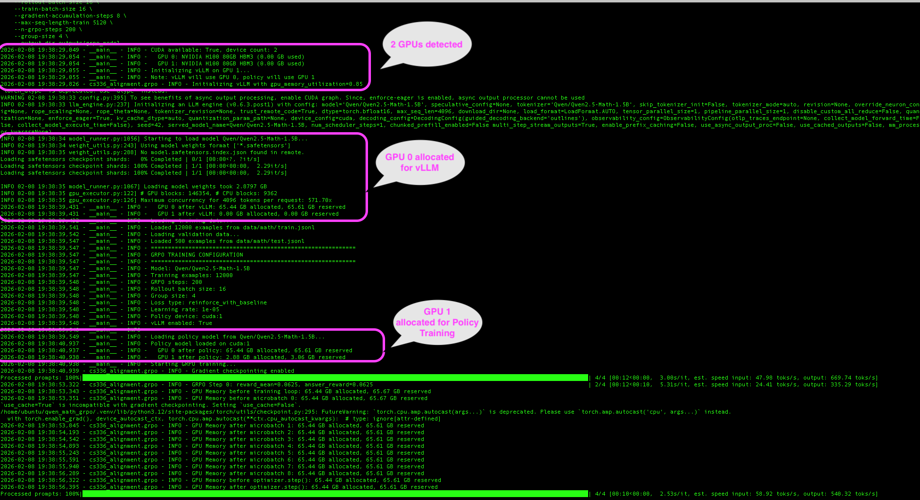
The 2-GPU architecture separates concerns. The screenshot below shows actual training logs from our Lambda Cloud run, with key moments annotated: detecting both H100 GPUs, vLLM claiming GPU 0 for fast rollout generation, and the policy model loading onto GPU 1 for training.

┌─────────────────────────────────────────────────────────────────────┐
│                   Lambda Cloud 2×H100 Setup                         │
├─────────────────────────────────────────────────────────────────────┤
│                                                                     │
│   GPU 0 (H100 80GB)              GPU 1 (H100 80GB)                  │
│   ┌─────────────────┐            ┌─────────────────┐                │
│   │                 │            │                 │                │
│   │     vLLM        │            │  Policy Model   │                │
│   │   (~65 GB)      │            │    (~3 GB)      │                │
│   │                 │            │                 │                │
│   │  - Fast batched │   sync     │  - Gradients    │                │
│   │    inference    │ ◄────────► │  - Optimizer    │                │
│   │  - KV cache     │  weights   │  - Backprop     │                │
│   │  - Continuous   │            │                 │                │
│   │    batching     │            │                 │                │
│   │                 │            │                 │                │
│   └─────────────────┘            └─────────────────┘                │
│                                                                     │
│   Rollout generation             Policy training                    │
│   (inference only)               (train mode)                       │
│                                                                     │
└─────────────────────────────────────────────────────────────────────┘

Understanding the hardware: A Lambda Cloud instance with 2×H100 GPUs also includes a host CPU (typically AMD EPYC or Intel Xeon) that orchestrates all work. The GPUs are accelerators—the CPU runs your Python code, loads data, and dispatches compute-heavy operations to the GPUs.

┌─────────────────────────────────────────────────────────────────────┐
│                    Lambda Cloud Instance                            │
├─────────────────────────────────────────────────────────────────────┤
│                                                                     │
│   ┌──────────────────────────────────────────────────────────────┐  │
│   │                      CPU (Host)                              │  │
│   │   • Runs Python/PyTorch orchestration code                   │  │
│   │   • Reward calculation (string parsing, regex)               │  │
│   │   • Advantage computation (simple arithmetic)                │  │
│   │   • Data loading and preprocessing                           │  │
│   └──────────────────────────────────────────────────────────────┘  │
│                          │                                          │
│            ┌─────────────┴─────────────┐                            │
│            ▼                           ▼                            │
│   ┌─────────────────┐         ┌─────────────────┐                   │
│   │    GPU 0        │         │    GPU 1        │                   │
│   │   (H100 80GB)   │         │   (H100 80GB)   │                   │
│   │                 │         │                 │                   │
│   │  vLLM rollouts  │         │ Policy training │                   │
│   │  (inference)    │         │ (forward/back)  │                   │
│   └─────────────────┘         └─────────────────┘                   │
│                                                                     │
└─────────────────────────────────────────────────────────────────────┘

Where does each step run?

Step	Location	What Happens
Rollout generation	GPU 0	vLLM generates G responses per question
Reward calculation	CPU	String parsing—extract answer, compare to ground truth
Advantage computation	CPU	Simple arithmetic: (r - μ) / (σ + ε)
Policy forward/backward	GPU 1	Compute log-probs and gradients
Optimizer step	GPU 1	Update weights with AdamW
Weight sync	GPU 0 ← GPU 1	Copy updated weights to vLLM

Benefits:

• No memory contention between inference and training
• vLLM can use continuous batching without interruption
• Policy model has dedicated memory for optimizer states
• Stable training with predictable memory usage

Step-by-Step Setup

1. Provision Instance

On Lambda Cloud, select an instance with 2+ GPUs:

• 2× A100 (80GB each) - recommended
• 2× H100 (80GB each) - faster, if available

2. SSH and Check GPUs

ssh ubuntu@<your-instance-ip>

# Verify GPUs are visible
nvidia-smi --list-gpus
# Expected: GPU 0: NVIDIA H100 80GB HBM3
#           GPU 1: NVIDIA H100 80GB HBM3

3. Install Dependencies

# Install uv package manager
curl -LsSf https://astral.sh/uv/install.sh | sh

# Clone and install
git clone https://github.com/bearbearyu1223/qwen_math_grpo.git
cd qwen_math_grpo
uv sync --extra vllm

4. Download Dataset

uv run python scripts/download_dataset.py

5. Run Training

uv run python scripts/run_grpo.py \
    --model-name-or-path Qwen/Qwen2.5-Math-1.5B \
    --rollout-batch-size 16 \
    --train-batch-size 16 \
    --gradient-accumulation-steps 8 \
    --max-seq-length-train 1024 \
    --n-grpo-steps 200 \
    --group-size 8 \
    --output-dir outputs/grpo_model

Parameter descriptions:

Parameter	Value	What It Does
--model-name-or-path	Qwen/Qwen2.5-Math-1.5B	Base model to fine-tune (downloaded from HuggingFace)
--rollout-batch-size	16	Number of questions sampled per GRPO step
--train-batch-size	16	Responses processed per gradient accumulation cycle
--gradient-accumulation-steps	8	Micro-batches accumulated before optimizer update
--max-seq-length-train	1024	Truncates prompt+response to this many tokens. Sequences longer than this limit are cut off. Lower values save GPU memory (activations scale with sequence length²) but may lose reasoning steps. For math problems, 1024 tokens typically covers the question + full solution.
--n-grpo-steps	200	Total training iterations
--group-size	8	Responses generated per question (G in the formula)
--output-dir	outputs/grpo_model	Where to save checkpoints and logs

How these numbers relate:

Questions per step:     16  (rollout-batch-size)
                        ×
Responses per question:  8  (group-size)
                        ═══
Total responses:       128  generated per GRPO step

Training processes:     16  (train-batch-size)
                        ×
Accumulation steps:      8  (gradient-accumulation-steps)
                        ═══
Effective batch:       128  responses per optimizer update

The numbers are chosen so all 128 generated responses are used in exactly one optimizer update. If you reduce rollout-batch-size or group-size, reduce the training side proportionally to match.

6. Download Results

# From your local machine
scp -r ubuntu@<your-instance-ip>:~/qwen_math_grpo/outputs ./lambda_outputs

Troubleshooting

Problem	Cause	Solution
CUDA out of memory	Batch size too large	Reduce --rollout-batch-size and --train-batch-size
Only 1 GPU detected	vLLM imported before torch	Check import order in code
OOM after manual termination of the training process	Zombie processes holding GPU memory	Run nvidia-smi --query-compute-apps=pid --format=csv,noheader \| xargs -I {} kill -9 {}
vLLM weight load fails	Wrong vLLM version	Ensure vLLM 0.6.x or 0.7.x (pinned in pyproject.toml)

Memory-saving parameters:

Parameter	Description	Reduce If OOM
--rollout-batch-size	Total responses generated per step	Yes
--train-batch-size	Samples processed per optimizer step	Yes
--gradient-accumulation-steps	Micro-batch size = train_batch / grad_accum	Increase (smaller micro-batches)
--max-seq-length-train	Truncate long sequences	Yes
--group-size	Rollouts per question	Yes

Interpreting Training Plots

After training, run plot_training.py to visualize metrics:

uv run python scripts/plot_training.py \
    --input outputs/grpo_model/training_history.json \
    --output training_plot.png

Here’s an example from our training run on Lambda Cloud:

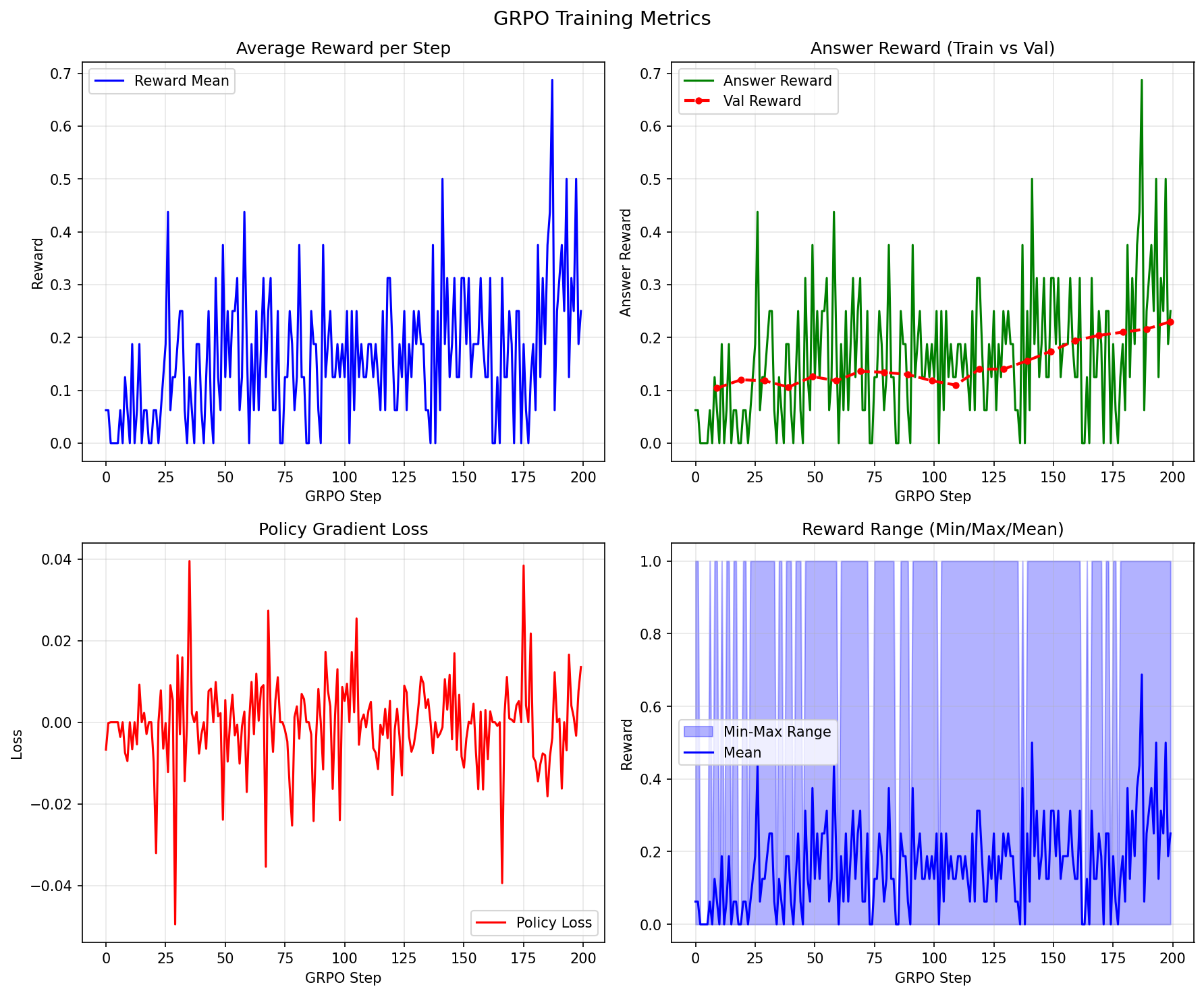
The plot has four panels. Here’s how to interpret each:

Panel 1: Average Reward per Step

What it shows: Mean reward across all responses generated at each GRPO step.

Healthy pattern:

• Gradual upward trend with noise
• Early steps: reward ~0.1-0.2 (model barely better than random)
• Later steps: reward ~0.3-0.5 (model learning)

Problematic patterns:

• Flat line: No learning (check rewards, advantages)
• Wild oscillations: Learning rate too high
• Sudden drops: Policy collapse (reduce learning rate or cliprange)

Healthy:                     Problematic (flat):
   ▲                            ▲
   │     ....●●●●               │ ●●●●●●●●●●●●●●●●●●●●●●●●
   │  ...●●                     │
   │ ●●●                        │
   └────────────────► step      └────────────────────► step

Panel 2: Answer Reward (Train vs Val)

What it shows: Accuracy on training data (green) and validation data (red).

Healthy pattern:

• Both curves trending upward
• Validation slightly below training (normal generalization gap)
• In our run: 6% → 25% accuracy (4× improvement!)

Problematic patterns:

• Train rising, val flat: Overfitting
• Both flat: Not learning
• Val higher than train: Data leakage or evaluation bug

Panel 3: Policy Gradient Loss

What it shows: The loss value from the policy gradient objective.

Healthy pattern:

• Generally decreasing trend with significant noise
• Fluctuations are normal (policy gradient has high variance)
• Should stabilize, not diverge

Problematic patterns:

• NaN values: Numerical instability (reduce learning rate)
• Steadily increasing: Wrong sign or bug
• Extremely low variance: Collapsed policy

Panel 4: Reward Range (Min/Max/Mean)

What it shows: For each training step, this panel plots three values:

• Max reward (top of blue area): The best response in the batch (usually 1 = correct)
• Min reward (bottom of blue area): The worst response in the batch (usually 0 = wrong)
• Mean reward (green line): Average reward across all responses

Why this matters for GRPO:

Remember, GRPO learns by comparing responses within a group. If the model generates 8 responses to a question:

Diverse (good for learning):        Uniform (no learning signal):
┌─────────────────────────┐         ┌─────────────────────────┐
│ Response 1: ✓ (r=1)     │         │ Response 1: ✗ (r=0)     │
│ Response 2: ✗ (r=0)     │         │ Response 2: ✗ (r=0)     │
│ Response 3: ✓ (r=1)     │         │ Response 3: ✗ (r=0)     │
│ Response 4: ✗ (r=0)     │         │ Response 4: ✗ (r=0)     │
│ ...                     │         │ ...                     │
│ min=0, max=1, mean=0.5  │         │ min=0, max=0, mean=0    │
│                         │         │                         │
│ → Advantages exist!     │         │ → All advantages = 0    │
│ → Model can learn       │         │ → Nothing to learn from │
└─────────────────────────┘         └─────────────────────────┘

Healthy pattern:

• Blue shaded area spans from 0 to 1 → Some responses correct, some wrong
• Mean line gradually rises → Model getting better over time
• Gap between min and max persists → Model is still exploring, still learning

Problematic patterns:

Pattern	What You See	What It Means	Fix
Range collapsed to 0	Blue area stuck at bottom	All responses wrong, no correct examples to reinforce	Problems too hard, or temperature too low (model not exploring)
Range collapsed to 1	Blue area stuck at top	All responses correct, nothing to discourage	Problems too easy, no learning signal
Mean not rising	Green line flat	Model not improving despite having diverse responses	Check loss function, learning rate, or reward calculation

Evaluation Results: Base Model vs GRPO-Trained

After training, we evaluated both the base Qwen2.5-Math-1.5B model and our GRPO-trained model on 500 math problems from the MATH dataset. Here’s the comparison:

Metric	Base Model	GRPO Model	Change
Correct answers	69 (13.8%)	205 (41.0%)	+136 (+197%)
Correct format, wrong answer	122 (24.4%)	170 (34.0%)	+48
Bad format (couldn’t parse)	309 (61.8%)	125 (25.0%)	-184

Key improvements:

1. 3× accuracy improvement — From 13.8% to 41.0% correct answers
2. Format compliance — Bad format responses dropped from 61.8% to 25.0%
3. Learning to reason — The model learned to show work and box final answers

Example improvements

Problem 1: Polar coordinates

Convert the point $(0, -3 \sqrt{3}, 3)$ from rectangular to spherical coordinates.

• Base model: $(6, \frac{2\pi}{3}, \pi)$ ❌ (wrong angles, no \boxed{})
• GRPO model: $\boxed{(6, \frac{5\pi}{3}, \frac{2\pi}{3})}$ ✓ (correct, properly boxed)

Problem 2: Double sum

Compute $\sum_{j = 0}^\infty \sum_{k = 0}^\infty 2^{-3k - j - (k + j)^2}$.

• Base model: $\frac{4}{3}$ ❌ (no work shown, unboxed)
• GRPO model: Step-by-step derivation → $\boxed{\frac{4}{3}}$ ✓

Problem 3: Function evaluation

Given $f(x) = \frac{x^5-1}{3}$, find $f^{-1}(-31/96)$.

• Base model: $-31/96$ ❌ (returned input, not inverse)
• GRPO model: Derived inverse function → $\boxed{\frac{1}{2}}$ ✓

These examples show that GRPO training taught the model to:

• Follow the expected format (\boxed{} for final answers)
• Show intermediate reasoning steps
• Actually compute answers rather than pattern-matching

Summary and Key Takeaways

Concept	Implementation	Why It Matters
Group normalization	A = (r - μ) / σ computed per question	Natural baseline without value network
Response masking	Loss computed on response tokens only	Don’t reinforce the prompt
2-GPU architecture	vLLM on GPU 0, policy on GPU 1	Avoid memory contention
Gradient checkpointing	policy.gradient_checkpointing_enable()	Reduce memory 2-3×
Off-policy training	Multiple gradient steps per rollout batch	More efficient data usage

Quick reference - key hyperparameters:

Parameter	Default	Effect
group_size (G)	8	More diversity → better baseline estimates
learning_rate	1e-5	Higher → faster but unstable
cliprange (ε)	0.2	Higher → more aggressive updates
gradient_accumulation_steps	128	Higher → more stable gradients
epochs_per_rollout_batch	1	Higher → more off-policy (needs clipping)

Next steps :

1. Experiment: Try different group sizes (4, 8, 16) and compare learning curves
2. Extend: Add your own reward functions for different tasks
3. Scale up: Try larger models (7B) with 4-GPU setups — larger models have more capacity to learn complex reasoning patterns and often start with stronger base capabilities. A 7B model needs ~14GB for weights alone, plus ~28GB for optimizer states, so you’ll need 4 GPUs: 2 for vLLM inference (tensor parallelism) and 2 for policy training

The math may seem daunting, but the core ideas are simple: sample multiple responses, compare them to each other, reinforce the good ones and avoid the bad ones. That’s really all there is to GRPO!

---

Resources:

• GRPO Training Code (this note’s implementation)
• MATH Dataset on HuggingFace — 12,500 competition math problems
• DeepSeekMath Paper — Original GRPO formulation
• DeepSeek-R1 Paper — GRPO at scale
• Stanford CS336: Language Modeling from Scratch
• Lambda Cloud — GPU instances for training