LLM Architecture Refresh [1]: Inside a Transformer Block — Attention, Heads, and the FFN
Taking a transformer block apart and measuring every piece — what attention computes and what it costs, why heads are a reshape rather than extra machinery, why the FFN is where a model keeps what it knows, and why the 1/sqrt(d_k) factor and RoPE are there at all.
Taking a transformer block apart, one measurement at a time
I can draw a transformer block from memory. For a long time I still couldn’t have told you which parts of it are actually expensive, why there’s a feed-forward network in there at all, or what that $1/\sqrt{d_k}$ is really doing. I’d absorbed the names without the reasons — and the usual explanations hand you more names.
So this post takes one block apart and puts a number on every piece.
The short version
If you read nothing else, these are the things this post establishes — each one measured rather than asserted:
- Attention is a weighted average, nothing more exotic. Each token looks at the others and pulls in a blend of what they offer, weighted by how relevant each one is. It is the only step in the entire model where tokens see each other at all.
- Extra heads are almost free. Splitting attention into 32 parallel copies costs the same parameters and the same arithmetic as running it once — it’s a reshape of a fixed budget, not extra machinery. What you buy is several opinions at once instead of one blurred compromise. The one cost that does grow with head count is the grid of token-against-token scores — a scratch value, discarded as soon as attention finishes, which at an 8k context still reaches 8 GiB per layer.
- What makes attention expensive is how wide the model is and how many tokens you feed it — not the head count. And the famous quadratic term is smaller than its reputation: at a 1,024-token sequence it’s 6% of the layer, while plain matrix multiplies are 89%.
- Attention can average, but it cannot conclude. Blending two facts never produces a third. That’s why every block also has a feed-forward network — the only part that transforms a token on its own, shaped like a lookup table, and where a model’s facts actually live.
- The $\sqrt{d_k}$ is not about overflow. It keeps the softmax in a range where a gradient still flows back, so how wide you make the heads stays a free choice instead of silently breaking training.
- RoPE gets relative position out of absolute rotation. Spin each token’s query and key by an angle set by its position, and the score between any two tokens ends up depending only on the gap between them — with no learned parameters at all.
- Training and serving are different jobs. Same model, 3× the arithmetic and 8× the memory to train: 16 GB to serve, 128 GB before a single activation. And what limits serving turns out to be the KV cache rather than the weights — about 1 GiB per 8k sequence, four times smaller than it would be without grouped-query attention.
Every one of those has a receipt behind it — a small program that prints the number, so you can check it rather than take my word. The code lives in a companion repo and runs unchanged on Apple Silicon or a Linux + NVIDIA box:
1
2
3
git clone https://github.com/bearbearyu1223/llm-architectures-refresher
cd llm-architectures-refresher
uv sync && uv run demo01
Every number and figure below came out of that command on my M-series Mac. The Python shown alongside each result is the part that matters, trimmed of setup — the runnable version is in demos/d01_attention.py.
Table of Contents
Skip to the short version for the findings without the derivations.
- What a language model actually does
- What attention is for
- The formula, symbol by symbol
- What a “head” is
- What attention costs
- What the whole model costs to run
- Following the shapes
- The rest of the block
- The FFN: where the model knows things
- The implementation, in five lines
- Why divide by sqrt(d_k)?
- Causal masking
- How this becomes learning, and becomes writing
- RoPE: absolute rotation, relative score
- A silent MPS bug that deleted RoPE
Plus a closing sidebar: the probe and an appendix of all notation.
1. What a language model actually does
Before attention, the thing attention is part of.
A language model does one thing: given some tokens, predict the next one. To write a sentence it does that over and over — predict a token, stick it on the end, feed the whole thing back in, predict again. All the sophistication is in how that single prediction gets computed.
That computation is a transformer: a stack of $L$ identical blocks — 32 of them in Llama-3-8B, for example — that a token’s numbers pass through in order, edited a little by each. Every block does exactly two things:
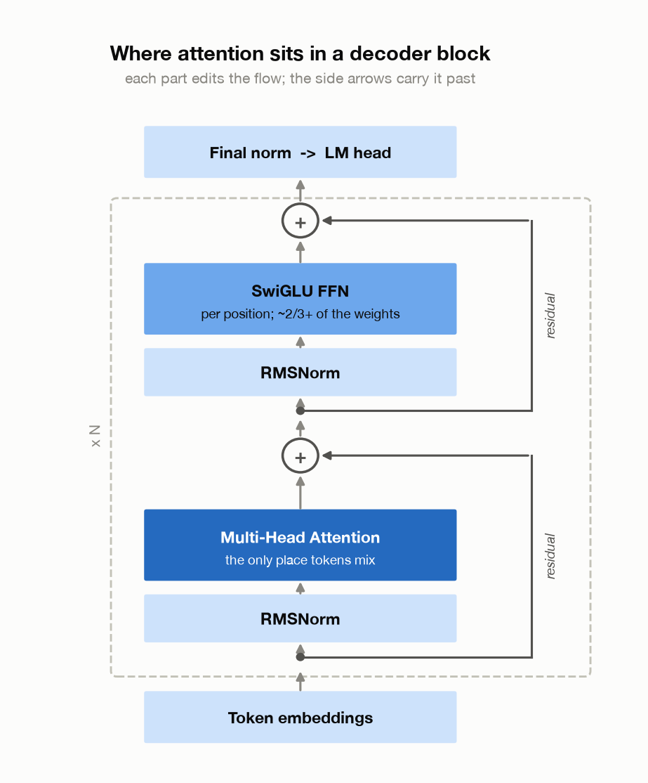
- Attention — each token looks at the other tokens and pulls in whatever it needs. This is the only step where tokens see each other.
- A feed-forward network (FFN) — each token, now holding some context, gets transformed on its own. No looking around.
Gather, then think. Thirty-two times over. At the end, one more layer turns a token’s numbers into a probability for every word in the vocabulary, and you pick one — §13 opens that layer up.
This post takes the whole block apart, in the order the vocabulary allows. Step 1 comes first and gets the most space — attention is where most of the design decisions are, and the rest is easier to describe once it’s in hand. Then §8 returns for the norms, those side arrows, and the “pre-norm” arrangement they add up to; §9 for the FFN, which holds more of a model’s parameters than attention does; and §13 for the loop itself — how a stack of per-token machinery ends up learning from a sequence, and writing one.
Numbers throughout this post come from one real model, Llama-3-8B, so they’re a checkable config rather than placeholders:
| Llama-3-8B | What it is | |
|---|---|---|
| $d_{model}$ | 4096 | how many numbers describe one token |
| $n_{vocab}$ | 128256 | how many distinct tokens the model knows (§8) |
| $n_{heads}$ | 32 | how many attention heads (§4) |
| $d_{head}$ | 128 | width of one head’s slice |
| $n_{kv}$ | 8 | key/value heads — fewer than query heads (§7) |
| $d_{ff}$ | 14336 | width of the FFN’s middle layer (§9) |
| $L$ | 32 | how many blocks are stacked |
These are one model’s choices, not universal constants: GPT-2 XL had $d_{model} = 1600$, split across 25 heads of 64 each. One relationship is universal, though — it holds for both models, and it does a lot of work later:
\[d_{model} = n_{heads} \times d_{head} \qquad 4096 = 32 \times 128\]For simplicity, §4 and §5 assume every query head has its own key and value head — 32 of each. That’s multi-head attention, or MHA. Llama-3-8B actually shares 8 key/value heads across its 32 query heads; §7 covers what changes.
2. What attention is for
A language model reads a sequence of tokens and builds a representation of each one. The hard part: a token’s meaning depends on other tokens, sometimes far away.
“The trophy didn’t fit in the suitcase because it was too big.”
Resolving it means looking back at two candidate nouns and picking one. A model that processes each token in isolation cannot do this at all.
Attention lets a token go and get information from other tokens, and learn which ones to get it from. For each token it computes a weight over every other token, then returns a weighted average of what those tokens offer. Relevant tokens get large weights; the rest get weights near zero.
Each token produces three vectors for this, from three learned projections:
| The question it answers | Its role | |
|---|---|---|
| Query $Q$ | “What am I looking for?” | the token doing the looking |
| Key $K$ | “What am I?” | how a token advertises itself |
| Value $V$ | “What do I contribute if chosen?” | the content actually retrieved |
A useful analogy: attention is a Python dictionary with fuzzy matching. A normal lookup tests keys for equality and returns one value. Attention replaces equality with a dot product (how aligned are they?) and replaces one value with a weighted average of all of them. That softness is the whole trick — a hard lookup has no gradient, so nothing could be learned.
3. The formula, symbol by symbol
Before the equation, the symbols in it:
| Symbol | What it is | Shape |
|---|---|---|
| $n$ | how many tokens are in the sequence | — |
| $d_k$ | how many numbers describe one query or key | — |
| $Q$ | the queries, one row per token | $(n, d_k)$ |
| $K$ | the keys, one row per token | $(n, d_k)$ |
| $V$ | the values, one row per token | $(n, d_k)$ |
| $K^\top$ | $K$ flipped, so the matrix multiply lines up | $(d_k, n)$ |
| $M$ | the causal mask, added before the softmax (see below) | $(n, n)$ |
With those in hand:
\[\text{Attention}(Q, K, V) = \text{softmax}\!\left(\frac{QK^\top}{\sqrt{d_k}}\right)V\]Read it from the inside out:
- $QK^\top$ — every query dotted with every key, giving an $n \times n$ grid of relevance scores. Row $i$ holds “how relevant is each token to token $i$?”
- $\div \sqrt{d_k}$ — a constant that keeps those scores in a sane range. §11 is devoted to why.
- $\text{softmax}$ — turns each row of scores into weights that are positive and sum to 1.
- $\times V$ — uses those weights to average the values, giving each token its answer.
The piece that formula is missing: the mask
As written, that equation lets every token see every other token — including the ones that come after it. For an encoder like BERT that’s exactly right. For a model that generates text it’s cheating: predicting token 5 while looking at token 6 isn’t prediction.
So decoder-only models add one more term, a mask $M$:
\[\text{Attention}(Q, K, V) = \text{softmax}\!\left(\frac{QK^\top}{\sqrt{d_k}} + M\right)V\]$M$ is an $n \times n$ matrix holding 0 where a position is allowed and $-\infty$ where it’s forbidden:
\[M_{ij} = \begin{cases} 0 & j \le i \quad \text{(token } j \text{ is at or before } i\text{)} \\[2pt] -\infty & j > i \quad \text{(token } j \text{ is in the future)} \end{cases}\]It’s rarely shown, so here it is for a 6-token sequence:
1
2
3
4
5
6
7
        key0     key1     key2     key3     key4     key5
  q0    0        -inf     -inf     -inf     -inf     -inf
  q1    0        0        -inf     -inf     -inf     -inf
  q2    0        0        0        -inf     -inf     -inf
  q3    0        0        0        0        -inf     -inf
  q4    0        0        0        0        0        -inf
  q5    0        0        0        0        0        0
Two details make this work, and both are the reason it’s written as an addition rather than a multiplication:
- $-\infty$, not a large negative number. Softmax exponentiates, and $e^{-\infty} = 0$ exactly. Forbidden positions get precisely zero weight, not merely a small one.
- It’s added before the softmax. So the surviving weights renormalize among themselves and each row still sums to 1. Masking after the softmax would leave rows summing to less than 1 — a classic bug.
Everything else in the formula is unchanged. §12 measures the result.
Two consequences to carry forward:
- The dot product is the only place tokens interact. Everything else in a transformer processes each token alone.
- The equation has no idea what order the tokens came in. Shuffle them and you get the same outputs, shuffled. Position must be injected separately — that’s §14.
4. What a “head” is
Running attention once has a limitation: a softmax produces exactly one set of weights — one opinion about which tokens matter. But a token usually needs several unrelated things at once: what noun this pronoun refers to, which verb governs this subject, which adjective modifies this noun. One weighting blurs them together.
The fix is to run attention several times in parallel, on different slices of the same vector — each copy free to form its own opinion.
What a head actually is
A head is one independent copy of attention, working on a 128-number slice of $Q$, $K$ and $V$. The order of operations matters, and it’s the detail most explanations blur:
- The token’s full 4,096-number vector is projected into $Q$, $K$, $V$. Each projection is $4096 \times 4096$, so $Q$, $K$ and $V$ are each 4,096 wide, and every number in them combines all 4,096 inputs.
- Then $Q$, $K$, $V$ are each cut into 32 slices of 128.
- Head $h$ takes slice $h$ of each and runs a complete attention pass.
- The 32 results are concatenated back to 4,096 and mixed by a final matrix $W_o$.
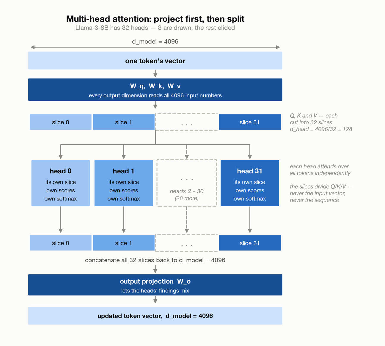
What gets sliced is $Q$/$K$/$V$, never the input. Two misreadings to head off, one per axis:
- Not the sequence. Every head sees every token. Head 3 doesn’t get “the last quarter of the sentence.”
- Not the input vector. Head 3 doesn’t get input dimensions 384–511 either. It gets dimensions 384–511 of $Q$, $K$, $V$, each computed from all 4,096 inputs.
Equivalently: head $h$ owns the 128 columns of $W_q$, $W_k$, $W_v$ that produce its slice, and those columns read the whole vector. That’s why you’ll see the mechanism described both ways — “project everything, then reshape” is what the code does; “each head has its own smaller projections” is what the math says.
$W_o$ at the end is not bookkeeping. Without it, 32 heads’ findings would sit in 32 disjoint stretches of the vector, unable to influence one another.
So what does all that buy? Several attention patterns at once, instead of one averaged compromise:
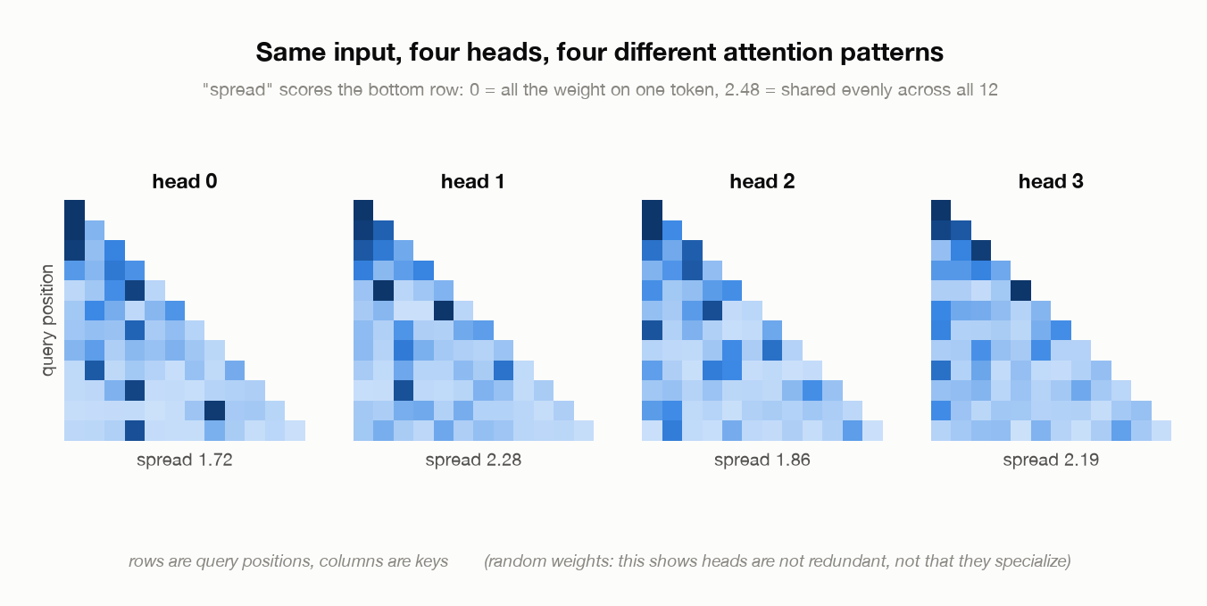
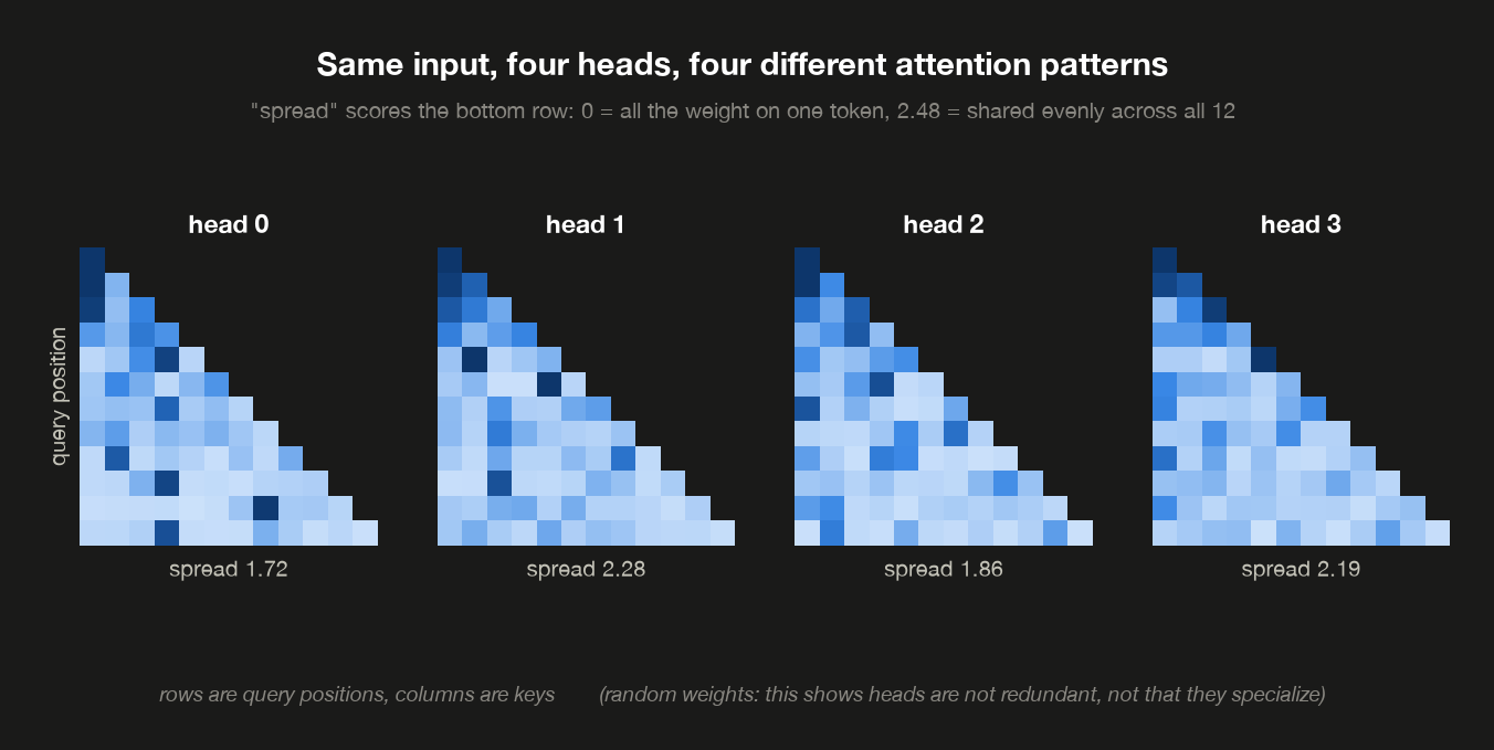
One triangle per head, all four fed the same 12 tokens. Read a triangle one row at a time: row $i$ is token $i$ doing the looking, and the cells along it are how much weight it puts on each token it can see — columns are those tokens, darker is more weight. The triangular shape is causal masking (§12): row $i$ stops at column $i$, because a token can’t look at anything to its right.
The thing to notice is that the four are not copies of each other. Compare their bottom rows — the last token’s view of the sentence, and the row that the number under each triangle summarizes. That number, spread, answers one question: is this row’s weight concentrated on a few tokens, or shared out across many? It’s the entropy of the row — a standard way to score how spread out a set of weights is. Put everything on a single token and it reads 0. Share it perfectly evenly across all 12 and it reads 2.48, the largest value possible here. Low means picky, high means even-handed, and the reason the ceiling is 2.48 rather than 12 is just that entropy is built from natural logarithms: $\ln 12 = 2.48$.
That also gives the number a concrete reading — undo the logarithm, and $e^{\text{spread}}$ is roughly how many tokens the row is effectively looking at. Head 0, at 1.72, is spreading itself over about 6 of the 12; head 1, at 2.28, over nearly 10. Same input, four different opinions.
One caveat I want to be exact about: these are random weights. The heads differ because they were initialized differently, which shows they aren’t redundant copies — it is not specialization. In trained models specialization is real and catalogued: “previous-token heads” that look one step back, “induction heads” that spot a repeated pattern and predict its continuation — both named and traced in Olsson et al., In-context Learning and Induction Heads (2022). You can’t see that in a figure like this.
So why not 512 heads? Because $n_{heads} \times d_{head}$ is fixed at $d_{model}$ — every head you add narrows all of them. At 32 heads each gets 128 numbers to describe a query; at 64 heads, 64 numbers; at 512, just 8, which is too few to express much of anything. A single head of 4,096 has the opposite problem: all the room in the world, and only one opinion. Models land at 32–64, where there are enough heads to disagree and enough width for each to have something to say.
5. What attention costs
The natural worry is that 32 heads means 32× the work. It doesn’t — but “heads are free” would be the wrong lesson, because attention is not cheap. It’s just that the head count isn’t what makes it expensive.
Two things do:
- $d_{model}$ — how wide a token’s vector is. The 4,096 numbers the embedding table hands over, carried unchanged through every block. Wider model, wider everything.
- $seq$ — how many tokens you are running through right now. Not the model’s advertised context window, which is only a ceiling. Feed a 128k-window model a 300-token prompt and every formula below uses $seq = 300$, not 128,000 — headroom you don’t use costs nothing. (Where that ceiling comes from in the first place turns out to be a RoPE question, so it waits for §14.)
Here is where every cost in an attention layer comes from:
| Cost | Kind | Formula | Grows with | Set by head count? |
|---|---|---|---|---|
| the projection matrices | memory | $4 d_{model}^2$ | vector width, squared | no |
| applying them | compute | $2 \cdot seq \cdot d_{model}^2$ | tokens × width² | no |
| computing the scores | compute | $2 \cdot seq^2 \cdot d_{model}$ | tokens squared × width | no |
| holding the scores | memory | $n_{heads} \cdot seq^2$ | tokens squared × head count | yes |
Two costs of each kind, and they are not interchangeable. Compute is work the chip has to do; memory is bytes it has to hold. On real hardware they run out at different times. Each kind has its own unit, and both get defined below before anything is counted with them: compute in FLOPs, memory in bytes. Note that the memory formulas count numbers, not bytes — converting between the two is the first aside. Three of the four don’t mention $n_{heads}$ at all, which is what makes the head count a free architectural choice; the fourth is a genuine exception.
Parameters. How wide does $W_q$’s output need to be?
It has to hand every head one slice of queries. With 32 heads of 128 that’s $32 \times 128 = 4096$ numbers — the same width as the input it started from. So $W_q$ takes 4,096 numbers in and produces 4,096 out: a $4096 \times 4096$ matrix.
Now change the head count and watch what happens. With 64 heads, each slice is only 64 numbers wide — but $64 \times 64 = 4096$ again. With 8 heads, each slice is 512 wide, and $8 \times 512 = 4096$. The output width never moves, because the head count and the head width always multiply back to $d_{model}$.
So $W_q$ is $4096 \times 4096$ no matter how many heads you choose, and the same holds for $W_k$, $W_v$ and $W_o$:
1
2
3
4
5
6
7
  matrix                         maps         shape  params
  -----------------------------------------------------------
  W_q     d_model -> n_heads x d_head  (4096, 4096)   16.8M
  W_k     d_model -> n_heads x d_head  (4096, 4096)   16.8M
  W_v     d_model -> n_heads x d_head  (4096, 4096)   16.8M
  W_o     n_heads x d_head -> d_model  (4096, 4096)   16.8M
  total                                               67.1M
$4096^2 = 16.8\text{M}$ per matrix, four matrices, $67.1$M per block — for any head count. Nothing in that arithmetic mentions $n_{heads}$. Note also that every matrix has 4,096 rows — the shape-level version of the point from §4, that each head reads the whole vector.
An aside: what those 67.1M numbers weigh
That figure counts numbers, not bytes — and the distance between the two is a deployment choice rather than an architectural one. One rule converts:
\[\text{bytes} \;=\; (\text{how many numbers}) \times (\text{bytes per number})\]The multiplier is the precision you store them in, and the name gives it away: fp32 is 32-bit floating point — 32 bits per number, which is 4 bytes. Every format is named the same way, so the multiplier is only ever the bit count divided by 8.
Run attention’s four projections through the rule — the count first, from the four $4096 \times 4096$ matrices above:
\[4 \times 4096^2 = 67{,}108{,}864 \text{ numbers}\]1
2
3
4
5
6
stored as sign/exp/frac bits bytes each total bytes weighs
------------------------------------------------------------------
fp32 1/8/23 32 4 268,435,456 256 MiB
bf16 1/8/7 16 2 134,217,728 128 MiB
fp16 1/5/10 16 2 134,217,728 128 MiB
fp8 1/4/3 8 1 67,108,864 64 MiB
Same architecture, down to a quarter of the memory, decided long after the model was designed. That’s why the memory rows in the table are written as counts: the count is fixed by the model, the multiplier is picked when you deploy it.
What those three groups of bits do. Floating point is binary scientific notation: a sign, an exponent and a fraction. That’s how one fixed budget of bits holds both enormous and tiny values. The exponent bits buy range: how large or small a number can get before it overflows to infinity or collapses to zero. The fraction bits buy precision: how many significant digits survive. That split is why training settled on bf16 rather than fp16 despite both being 16 bits — bf16 keeps all 8 of fp32’s exponent bits and gives up fraction instead, and gradients span enormous magnitudes, so a value that underflows to zero stops training that weight altogether, while a slightly imprecise one does little harm. (fp8 comes in two flavours for the same reason: the 1/4/3 split above, and a 1/5/2 variant that trades one more fraction bit for range.) The training breakdown further down uses exactly that trade: fp16 weights for speed, alongside an fp32 master copy so millions of tiny updates don’t vanish into rounding.
Those totals land on round numbers because every quantity here is a power of two. $4096 = 2^{12}$, so one matrix is $2^{24}$ numbers and four of them are $2^{26}$; at 4 bytes each that’s $2^{28}$ bytes, and since a MiB is $2^{20}$ bytes, the answer is exactly $2^8 = 256$ MiB. Worth watching the units, though — a MiB is $1024^2$ bytes while a MB is $10^6$, so those same weights are an unlovely 268.4 MB in the decimal units GPU spec sheets quote. This post stays in MiB until §6, where the comparison is against real cards and their decimal spec sheets.
One warning the capacity number hides. Memory bills you on two separate meters: how many bytes you have to hold, in GB, and how fast you can move them, in GB/s. The weights sit in the GPU’s memory while the arithmetic happens in its compute units, so every number has to make that trip — capacity decides whether the model runs at all, bandwidth decides how fast it runs. Two budgets, two ways to fail: miss the first and you get an out-of-memory error, miss the second and it runs correctly but slowly, with all that spare capacity doing nothing to help. §6 works through a decode step where the second meter, not the first, sets the token rate.
An aside: what a FLOP is, and how to count one
The other half of the cost is measured in FLOPs, so before using the word:
A FLOP is one floating-point operation — a single add or a single multiply on decimal numbers. “FLOPs” (lowercase s) counts operations; “FLOP/s” is a rate, operations per second. They look almost identical and mean different things: a model needs so many FLOPs, a GPU delivers so many FLOP/s, and dividing one by the other estimates time.
Counting them in a transformer is easy, because nearly all the arithmetic is matrix multiplication, and one rule covers every matmul:
\[(a, b) \times (b, c) \;\longrightarrow\; 2 \cdot a \cdot b \cdot c \;\text{ FLOPs}\]Where that comes from: the result has $a \times c$ entries, and each is a dot product of two length-$b$ vectors — $b$ multiplies and $b$ adds, so $2b$ operations. Multiply out and you get $2abc$. In words:
FLOPs = 2 × (number of output entries) × (length of the dimension being summed away).
The 2 is the multiply-and-add pair. Hardware runs them as one fused instruction, but the convention counts both.
That’s the whole method. It also hands you a rule of thumb. Each weight is used in one multiply-add per token, so a forward pass costs about $2N$ FLOPs per token, where $N$ is the parameter count.
Score FLOPs. Here the head count really does look like it should matter: 32 heads, each doing its own matrix multiply. It doesn’t, and for the same reason as before.
Inside one head, $QK^\top$ multiplies a $(seq, d_{head})$ matrix by a $(d_{head}, seq)$ one. Applying the rule from above — 2 × output entries × the dimension summed away:
\[\text{one head} \;=\; 2 \times seq^2 \times d_{head}\]Then there are $n_{heads}$ of them, so multiply through:
\[\text{all heads} \;=\; n_{heads} \times 2 \times seq^2 \times d_{head} \;=\; 2 \times seq^2 \times \underbrace{\big(n_{heads} \times d_{head}\big)}_{=\; d_{model}} \;=\; 2 \times seq^2 \times d_{model}\]The head count cancels, exactly as it did for the parameters — and for the same reason, that the two always multiply back to $d_{model}$. At $seq = 1024$:
1
2
3
4
5
6
  n_heads  d_head  n_heads x d_head  FLOPs per head  x n_heads = total
  ----------------------------------------------------------------------
  1          4096              4096          8.59 G             8.59 G
  8           512              4096          1.07 G             8.59 G
  32          128              4096          0.27 G             8.59 G
  64           64              4096          0.13 G             8.59 G
Read the last two columns together: halving $d_{head}$ halves the per-head cost, and doubling the head count multiplies it straight back. Going from 1 head to 64 makes each head 64× cheaper and there are 64× as many — exactly inverse, so the final column never moves.
So heads are a reshape of a fixed budget, not extra machinery. You’re only choosing whether to read the same 4,096 numbers as one wide space or many narrow ones.
Except in one place: the score matrix
That table had a fourth row, and it’s the honest exception. The scores live in a tensor of shape $(n_{heads}, seq, seq)$ — one $seq \times seq$ grid per head. Narrower heads make each dot product cheaper, which is why the FLOPs cancel; they do not make each grid smaller.
1
2
3
4
5
6
  n_heads  d_head  score FLOPs  score matrix (fp32)
  ---------------------------------------------------
  1          4096       8.59 G                4 MiB
  8           512       8.59 G               32 MiB
  32          128       8.59 G              128 MiB
  64           64       8.59 G              256 MiB
Identical arithmetic, 64× the activation memory.
Now, 128 MiB doesn’t sound alarming — but that’s at a 1,024-token sequence, and this term is quadratic. Stretch the context and it goes somewhere ridiculous:
1
2
3
4
5
6
  seq      score matrix (fp32)  vs 8B weights in bf16
  -----------------------------------------------------
  1,024                128 MiB                  0.01x
  8,192                  8 GiB                  0.53x
  32,768               128 GiB                  8.56x
  131,072                2 TiB                136.93x
Every figure there is per layer, per forward pass, and the model has 32 layers.
That last column is the one to hold on to. At an 8k context, one layer’s score matrix is 0.53× the size of every weight in the model — 8 GiB against 15 GiB in bf16, which is the quantity §6 quotes as 16.1 GB once you switch to the decimal units spec sheets use. At 128k a single layer reaches 137× the weights, which no accelerator on earth has.
And the reason to avoid this cost rather than budget for it: it’s scratch. The score matrix isn’t part of the model and isn’t part of the answer. It’s computed, softmaxed, multiplied by $V$, and thrown away microseconds later. Nothing wants it — it’s just an unavoidable-looking step on the way to the output.
Except training does want it. The backward pass needs those attention weights to compute gradients, so the obvious implementation has to keep every one of them alive until the backward pass arrives. That’s what turns a transient into a memory ceiling, and it kept long context impractical for years.
The escape is to compute attention in small tiles so the full grid never exists at once, and to recompute the pieces the backward pass needs instead of storing them — trading arithmetic, which is cheap, for memory traffic, which isn’t. That’s Flash Attention, and post 3 is entirely about it.
Where the FLOPs actually go
That table counted only $QK^\top$. Applying the same rule to every matmul in one attention layer gives the full picture — and it’s not what people expect:
1
2
3
4
5
6
  step                       shapes (32 heads)    FLOPs  share
  --------------------------------------------------------------
  W_q/W_k/W_v/W_o  4 x (1024,4096)@(4096,4096)  137.4 G    89%
  Q @ K.T           32 x (1024,128)@(128,1024)    8.6 G     6%
  weights @ V      32 x (1024,1024)@(1024,128)    8.6 G     6%
  total                                         154.6 G
Note the 32 × on the attention rows: those are thirty-two small matmuls, one per head, summed — not one big one. It happens not to change the total, because $32 \times 128 = 4096$ makes the arithmetic identical either way, but it is what actually runs.
One assumption to head off: grouped-query attention, the arrangement Llama-3-8B actually uses, doesn’t shrink these. Its 8 key/value heads are broadcast back up to 32 right before the matmul, so every query head still scores against a full-width key. GQA saves cache and parameters, not attention FLOPs — and §6 puts a number on the cache it does save.
The quadratic term is the smallest item here. At a 1,024-token sequence, attention’s famous $n^2$ cost is 6% of the layer; the four projections are 89%. The $n^2$ term only takes over once $seq$ grows past $d_{model}$ — below that, a transformer is mostly big dense matrix multiplies, and “attention is quadratic” describes the asymptote, not the regime most models run in. Post 3 is about what happens when you do cross that line.
The $2N$ rule of thumb checks out here too. It came out of the FLOP aside: every weight gets used in exactly one multiply-add per token, so a forward pass should cost about $2N$ FLOPs per token, where $N$ is the parameter count. Attention’s four projections hold $N = 67.1$M parameters, and this table pushes 1,024 tokens through them, so the rule predicts
\[2 \times 67{,}108{,}864 \times 1024 = 137.4 \text{ G FLOPs}\]which is the projection row of the table above, to the digit. The demo checks that equality rather than asking you to take it on trust — the last line is the comparison, not a label:
1
2
3
  projection params N                67.1M
  2 x N x tokens                     137.4 G
  equals the measured projection cost yes
(Everything above is head-count independent for the same reason as before.)
6. What the whole model costs to run
Everything so far has been one layer, priced in $d_{model}$ and $seq$. Now put the whole model on a card you could actually rent and ask the two questions that decide everything: does it fit, and how fast does it go?
One number carries the section, and it has just changed meaning:
1
2
  N, whole-model parameters          8.03B
  (not the 67.1M above — that was one layer's four projections)
The FLOP aside used $N$ for a single layer’s four projections. From here it means the whole model — all 32 blocks, plus the embedding table and the LM head: the two lookup tables sitting at either end of the stack, one turning a token into a vector on the way in, the other turning a vector back into scores over the whole vocabulary on the way out. §13 opens them up as a single table read in both directions; for now what matters is that they are large, and they are part of $N$.
The budget
One A100 80GB, with its successor alongside for contrast:
1
2
3
4
  GPU        memory  bandwidth  BF16 compute
  --------------------------------------------
  A100 80GB   80 GB  2.04 TB/s   312 TFLOP/s
  H100 80GB   80 GB  3.35 TB/s   990 TFLOP/s
Three columns, three different questions. Memory decides whether a job fits at all. Bandwidth decides how fast weights reach the arithmetic units. Compute decides how fast the arithmetic runs once they arrive. Take them in that order — the first is pass/fail, and the other two only matter once you’ve passed it.
One caveat before spending any of it: 80 GB is not 80 GB. The CUDA context, cuBLAS workspaces and allocator fragmentation take a few gigabytes before any tensor of yours lands, so budget against ~77 GB usable. Planning to the nominal number is how you meet fragmentation at 3 a.m.
Serving: the weights are only the floor
Weights are $N \times$ bytes-per-parameter — the bytes rule from §5, applied to all 8.03 billion instead of one layer’s 67.1M:
1
2
3
4
5
6
  stored as  bytes/param  weights
  ---------------------------------
  fp32                 4  32.1 GB
  bf16/fp16            2  16.1 GB
  int8                 1   8.0 GB
  int4               0.5   4.0 GB
At bf16 that’s 16.1 GB against 77 usable, so “can one card serve an 8B model” gets an easy yes. But weights are the floor, not the bill.
The ceiling is the KV cache
Generating text means keeping every key and value already computed, so the model doesn’t rebuild the whole prefix for each new token. That cache grows with every token, and its size is pure architecture:
\[2 \times L \times n_{kv} \times d_{head} \times \text{bytes per number}\]Two for K and V, $L = 32$ layers, $n_{kv} = 8$ key/value heads, $d_{head} = 128$, two bytes each in bf16:
1
2
3
  KV cache per token (GQA, 8 kv)     128 KiB
    had it been MHA (32 kv)          512 KiB — 4x worse
  KV per full 8k sequence            1.00 GiB
This is where GQA earns its keep, and it settles something §5 left open. There, GQA saved nothing on attention FLOPs, because its 8 key/value heads get broadcast back up to 32 before the matmul. Here is what it saves instead: the cache is sized by $n_{kv}$, not $n_{heads}$, so 8 instead of 32 makes it four times smaller. Had Llama 3 used plain MHA, one full 8k sequence would cost 4 GiB of cache rather than 1.
Remember 1 GiB per 8k sequence and you can convert spare memory straight into a concurrency number:
1
2
3
4
5
6
7
8
9
  card, nominal / usable             80 GB / ~77 GB
    minus weights, workspace         58 GB left for KV
    which buys                       ~442k tokens of cache

  context length  concurrent sequences
  --------------------------------------
  8k                               ~54
  32k                              ~13
  128k                              ~3
That last table is the real answer to “how many users can one card serve.” At 8k context, around 54 — a genuine server. At 128k, three. The binding constraint for serving is the KV cache at long context, not the weights, and post 2 is entirely about living with that.
How fast it generates
Memory said yes. Now the other two columns, which disagree violently. At batch 1 — a single stream, one token at a time — a decode step reads every weight exactly once, so you can time it two ways: by the arithmetic it does, or by the bytes it moves.
1
2
3
4
  GPU        if compute-bound  if bandwidth-bound   gap
  -------------------------------------------------------
  A100 80GB      19,427 tok/s           127 tok/s  153x
  H100 80GB      61,644 tok/s           209 tok/s  296x
Both columns are a single division. Take the H100 and an 8B model in bf16 — 16.1 GB of weights to move, and $2N \approx 16$ GFLOPs of arithmetic to do:
\[\text{bytes: } \frac{16.1\ \text{GB}}{3.35\ \text{TB/s}} \approx 4.8\ \text{ms} \;\longrightarrow\; 209\ \text{tok/s}\] \[\text{math: } \frac{16\ \text{GFLOP}}{990\ \text{TFLOP/s}} \approx 0.016\ \text{ms} \;\longrightarrow\; 61{,}644\ \text{tok/s}\]Neither number is the answer on its own. A chip can be doing arithmetic while bytes are still in flight, so the two overlap and the slower one sets the floor:
\[\text{time} \;\approx\; \max\!\left(\frac{\text{bytes}}{\text{bandwidth}},\;\; \frac{\text{FLOPs}}{\text{throughput}}\right)\]Compute both, take the larger, and that tells you which spec-sheet number you’re actually buying. It’s the roofline model in one line, it applies to any kernel rather than just decode, and it assumes the overlap is perfect — which is why real code lands above this floor rather than on it.
Bandwidth wins by two orders of magnitude. The chip multiplies for 16 microseconds, then waits roughly 4.8 milliseconds for the next weights to arrive — busy about 0.3% of the time. All those TFLOP/s are unreachable for this workload.
And it gets worse, not better: the H100 has 3.2× the compute of an A100 but only 1.6× the bandwidth, so the gap roughly doubles between generations. Buying a faster chip mostly buys compute you can’t use.
(Peak numbers; real kernels reach a fraction of them. Batching improves the picture a lot, and now it’s clear why — a batch of 64 reads each weight once and spends it on 64 tokens, so arithmetic done per byte moved rises with the batch size. That’s what continuous batching in vLLM or TensorRT-LLM is buying. But the ratio is what matters here, and it survives the discount.)
Training: the same model, eight times the memory
A tempting piece of arithmetic: 16.1 GB of weights, 77 GB of card, therefore training fits. It does not, and the gap isn’t close.
Compute first, since it’s the mild part. Training runs the model forward and then backward, and the backward pass costs about twice the forward one. On the way back, every layer has to answer two questions where on the way in it answered only one.
Going in, a layer has one job: take its input, produce its output. Coming back, it is handed a message — the output you produced was wrong; it should have been a little higher here, a little lower there — and from that one message it works out two different things:
- how its own weights should change, given that its output was wrong that way. This is the point of the whole exercise — though the backward pass only computes that correction. It gets stored, and a separate optimizer step applies it once the whole pass is done.
- what its input should have been, for that output to have come out right. It can’t act on this one — its input is whatever the previous layer handed over. But “what my input should have been” is the same statement as “what your output should have been” to the layer behind it, so this answer is the message that keeps the chain moving.
Each of those is a matrix multiply the same size as the forward one, so the way back costs two forward passes’ worth of arithmetic. It’s also why the backward pass is a chain rather than 32 independent calculations: a layer can’t start until the layer after it has produced that message. (§13 writes both multiplies out, if you want the algebra rather than the words.) Add the original forward pass and training comes to 3× inference, per token:
1
2
3
4
  per token        FLOPs                            why
  -------------------------------------------------------
  inference  2N = 16.1 G               one forward pass
  training   6N = 48.2 G  forward, then backward at ~2x
Three times the arithmetic. That part is mild. Memory is where the two jobs separate, because training has to keep the optimizer’s state beside the weights:
1
2
3
4
5
6
7
  what                   cost     size  running total
  -----------------------------------------------------
  bf16 weights      2 B/param  16.1 GB        16.1 GB
  bf16 gradients    2 B/param  16.1 GB        32.1 GB
  fp32 master copy  4 B/param  32.1 GB        64.2 GB
  Adam moment m     4 B/param  32.1 GB        96.4 GB
  Adam moment v     4 B/param  32.1 GB       128.5 GB
Those last four rows are the compute story made concrete. The gradients need 16.1 GB precisely because the backward pass computes corrections rather than applying them — they have to sit somewhere until the optimizer step runs. The fp32 master copy exists so millions of tiny updates don’t vanish into bf16’s seven fraction bits. Adam then keeps two running averages of past gradients, so each update is smoothed against recent history instead of following the raw gradient. None of it would exist if the backward pass simply changed weights as it went.
About 2 bytes per parameter to serve, about 16 to train. So:
1
2
  training state (16 B/param)        128 GB
    against usable                   77 GB — over by 51 GB
Over budget before a single activation is allocated. An 8× gap between serving and training, which is why a model that serves happily on one card needs several to fine-tune.
The two costs nobody budgets for
The 128 GB above is the part people remember. Two more get underestimated, and either can be the thing that actually triggers the out-of-memory error.
Activations. Inference discards each layer’s intermediate values as it goes; training cannot, because $dW = X^\top dY$ needs the layer’s input $X$ from the forward pass (§13 shows exactly which product is responsible). Left alone, that means every intermediate inside every block stays alive from the moment it is computed until the backward pass comes back for it — and they are not small. The FFN’s middle tensor alone is $4{,}096 \times 14{,}336$ numbers, 117 MB per block in bf16, 3.8 GB across all 32.
Gradient checkpointing is the escape, and the name is meant literally. You choose checkpoints through the network, here the input to each block, keep only those, and throw away everything computed in between. When the backward pass asks for something that was thrown away, that block is run forward a second time from its saved input to rebuild it. Storage drops to one tensor per block; the price is a second forward pass through every block, roughly 30% more compute overall.
That makes the surviving figure easy to predict: one saved tensor per block, each $seq \times d_{model}$, two bytes apiece.
\[32 \times 4{,}096 \times 4{,}096 \times 2 \text{ bytes} \;\approx\; 1.1 \text{ GB}\]which is what the demo prints. In its shorthand, ckpt means checkpointing is on, b is the batch size and s the sequence length:
1
    activations, ckpt b=1 s=4096     1.1 GB
The logits tensor, which is the sneaky one. The vocabulary is 128,256 wide, and training scores every position at once, so one 4,096-token sequence materialises a $4096 \times 128{,}256$ tensor:
1
    logits, fp32 at seq 4096         2.1 GB per sequence
Softmax and its gradient typically need two or three copies of that, so 4–6 GB for a single sequence — larger than several transformer blocks put together, from a layer that is conceptually just a lookup (§13 opens it up). On models with big vocabularies this is often the real OOM trigger rather than the optimizer. Fused and chunked cross-entropy implementations exist for exactly this.
The verdict
| Task | One A100 80GB? | What binds |
|---|---|---|
| bf16 inference | yes, easily | 16.1 GB of weights |
| inference at 8k context | yes | ~1 GiB of KV cache per sequence |
| int8 / int4 inference | yes, very easily | 8.0 / 4.0 GB of weights |
| full fine-tune, plain AdamW | no | 128 GB of training state |
| full fine-tune, with offload and 8-bit optimizer | borderline | fits via tricks, then PCIe-bound |
| pretraining from scratch | no, practically | compute, not memory |
So: 8 billion parameters does not mean an 8 GB model. The same architecture is 4–32 GB to serve depending on precision, and comfortably over 100 GB to train, because training adds gradients, master weights, optimizer moments and activations on top of the weights themselves.
Why pretraining is a different question entirely
Everything above is a memory question, and memory questions have engineering answers — shard the optimizer state across GPUs and 128 GB becomes 16 GB on each of eight cards.
Pretraining is a compute question, and it doesn’t yield to the same trick. The table above says a training token costs $6N$ FLOPs. Multiply by however many tokens you intend to train on and you get the whole bill:
\[C \approx 6ND\]That’s the entire budget for a training run, and it is the $6N$ from this section with $D$ tokens pushed through it. Llama 3 was trained on more than 15 trillion, per Meta’s model card:
\[6 \times 8.03\text{B} \times 15\text{T} \approx 7.2 \times 10^{23} \text{ FLOPs}\]Meta reports roughly 1.3 million H100-hours for the 8B model, which is about 148 GPU-years on a single card — and an A100 is materially slower than an H100. No amount of memory tricks touches that number.
Which is the thing to end on. You don’t need thousands of GPUs because the model won’t fit; sharding solves that with eight. You need thousands because there are trillions of tokens to push through it, and the only way to buy wall-clock time is to run them in parallel.
Both posts that follow are about memory rather than math. Post 2 is about the cost this section just met — the KV cache that decides how many sequences a card can serve. Post 3 is about the score matrix from §5: the $seq \times seq$ grid, and how to get attention’s answer without ever writing it down.
7. Following the shapes
Shapes are where most confusion about attention lives. Rather than write a table by hand — easy to get subtly wrong — the demo runs a real attention module on a 10-token prompt and prints what PyTorch reports. This is the code it runs:
1
2
3
4
5
6
7
8
9
10
11
12
q, k, v = x @ w_q, x @ w_k, x @ w_v                    # (seq, 4096) each

# split into heads: view, then move the head axis to the front
qh, kh, vh = (t.view(seq, n_heads, d_head).transpose(0, 1)
              for t in (q, k, v))                      # (32, seq, 128)

scores = (qh @ kh.transpose(-2, -1)) / math.sqrt(d_head)   # (32, seq, seq)
weights = torch.softmax(scores.masked_fill(mask, float("-inf")), dim=-1)
ctx = weights @ vh                                     # (32, seq, 128)

merged = ctx.transpose(0, 1).reshape(seq, d_model)     # (seq, 4096)
out = merged @ w_o                                     # (seq, 4096)
Note the .transpose(0, 1) on line 4: that’s what makes the head axis come first. And what PyTorch reports for each step:
1
2
3
4
5
6
7
8
9
10
11
12
13
14
15
16
17
18
  classic multi-head attention (MHA): one K and V head per query head
  seq=10, d_model=4096, n_heads=32, d_head=128

  tensor                             shape                          note
  ------------------------------------------------------------------------
  x   (the token vectors)       (10, 4096)             one row per token
  W_q, W_k, W_v               (4096, 4096)     each reads all of d_model
  Q, K, V  after projection     (10, 4096)              still full width
  Q, K, V  split into heads  (32, 10, 128)               4096 = 32 x 128
  one head's Q                   (10, 128)  what the formula operates on
  scores = Q Kt / sqrt(d_k)   (32, 10, 10)    per head, quadratic in seq
  weights  after softmax      (32, 10, 10)            each row sums to 1
  weights @ V                (32, 10, 128)               per-head answer
  concatenated heads            (10, 4096)            back to full width
  output  after W_o             (10, 4096)       same shape as the input

  input and output shapes match      yes
  attention weights row sum          1.0000
Three things fall out:
- The module is shape-preserving. In at
(10, 4096), out at(10, 4096)— which is exactly what makes blocks stackable. - Only the score matrix depends on $n^2$. At
seq=10it’s a nuisance; atseq=128000it’s the whole problem, which is post 3. - $W_q$ is square. It shrinks nothing. The reshape does the splitting; the matrix only mixes.
How to picture (32, 10, 128)
Three-axis shapes are where notation stops being readable. The image that works: a deck of 32 sheets, each sheet a 10 × 128 table — 10 rows, one per token; 128 columns, that head’s features.
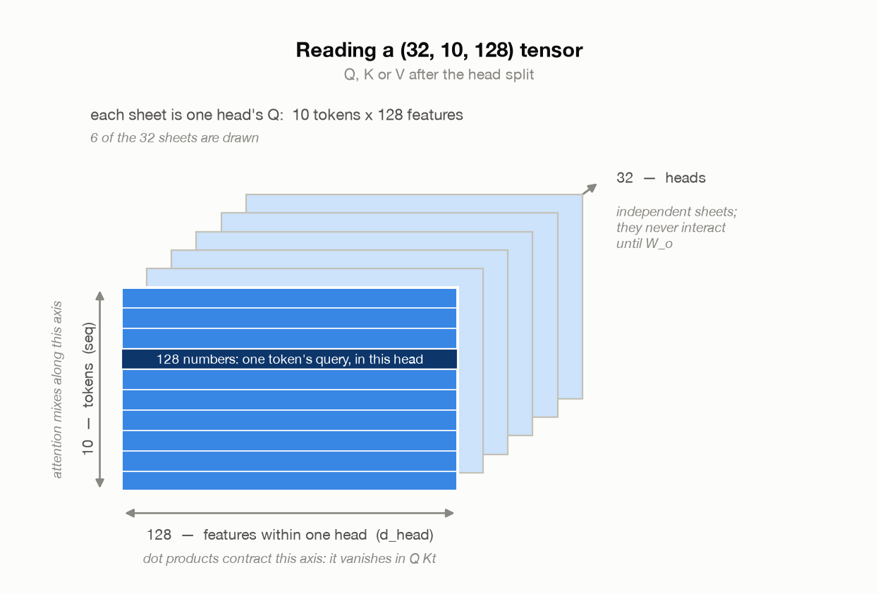
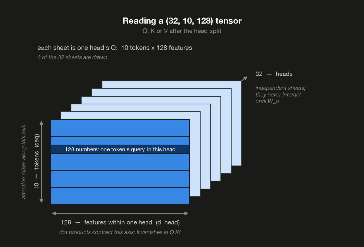
Resist drawing it as a solid cuboid. A cuboid suggests the three axes are interchangeable directions, and they aren’t — each axis has a different job:
| Axis | Size | What happens along it |
|---|---|---|
| heads | 32 | Nothing. Pure parallelism; sheets never interact until $W_o$ |
| tokens | 10 | Attention mixes along this axis — the only one that gets mixed |
| features | 128 | Dot products contract this axis — it disappears in $QK^\top$ |
That last row explains the shape changes people find most confusing. One rule does all the work:
A matrix multiply contracts the shared inner dimension. $(a, b) \times (b, c)$ gives $(a, c)$, and $b$ is summed away.
Attention applies it twice, and the two are mirror images:
1
2
3
4
  step              left      right     output  axis summed away
  ----------------------------------------------------------------
  Q @ K.T      (10, 128)  (128, 10)   (10, 10)    128 (features)
  weights @ V   (10, 10)  (10, 128)  (10, 128)         10 (keys)
First matmul: the 128 features are summed away and a second token axis appears. You’ve turned “each token’s features” into “each token’s relevance to each other token.”
Second matmul: the 10 keys are summed away and V’s 128 features come back. This is the step whose output shape surprises people: weights is $(10, 10)$ and V is $(10, 128)$, so the shared axis is tokens, leaving one row per query and 128 columns from V. Written out, output row $i$ is literally a weighted sum of V’s rows:
Ten weights, ten value-vectors of 128 numbers each, one 128-number result. That’s why the answer is 128 wide rather than 10 wide — the weights say how much of each token to take, and V says what to take.
Worth checking that claim rather than taking it. Pick any single output row — say head 0, query position 3 — and compute it two ways: once as the library does it, and once literally as the sum above, looping over tokens.
1
2
from_matmul = (weights @ V)[0, 3]                                  # the matmul
by_hand = sum(weights[0, 3, j] * V[0, j] for j in range(seq))      # the definition
Both should be the same 128 numbers. Their first four:
1
2
3
4
    from the matmul                  +0.5989  -0.0095  -0.3333  -0.4037
    from the by-hand sum             +0.5989  -0.0095  -0.3333  -0.4037

  largest disagreement, all 128      1.788e-07
Agreement to 1.8e-07 across all 128 — float noise, not a real difference. The matmul is the weighted sum, written as one operation instead of a loop. Which is the point: weights @ V looks like opaque linear algebra, and it’s doing exactly the “take 70% of this token, 20% of that one” averaging from §2.
What changes with grouped-query attention
Here’s the simplification promised in §1. Everything above is classic multi-head attention, where every query head gets its own key and value head. Llama-3-8B instead uses grouped-query attention: 32 query heads sharing only 8 key/value heads, so its $K$ and $V$ projections are a quarter as wide:
1
2
3
4
5
6
  tensor                  MHA (32 kv heads)  Llama-3-8B (8 kv heads)
  --------------------------------------------------------------------
  W_q                          (4096, 4096)             (4096, 4096)
  W_k, W_v                     (4096, 4096)             (4096, 1024)
  Q  split into heads         (32, 10, 128)            (32, 10, 128)
  K, V  split into heads      (32, 10, 128)             (8, 10, 128)
Each projection still follows one rule — it is $(d_{model},\; \text{heads it feeds} \times d_{head})$ — so 8 key heads of 128 gives $(4096, 1024)$. That drops the block’s attention parameters from 67.1M to 41.9M.
Note the asymmetry: $Q$ keeps full width; only $K$ and $V$ shrink. That’s deliberate — $K$ and $V$ are the tensors generation has to cache, so shrinking them shrinks the memory that limits how many users you can serve. $Q$ is recomputed every step and never cached. Post 2 is largely about this.
Read the rest of this post as classic MHA; the mechanism is identical either way.
8. The rest of the block
Back to the diagram from §1. Attention was one box in it. Here are the others — and the wrapping around all of them.
Inside the attention box
Start with the box this post has been about. Here’s the data path inside it, with the tensor’s shape down the right margin:
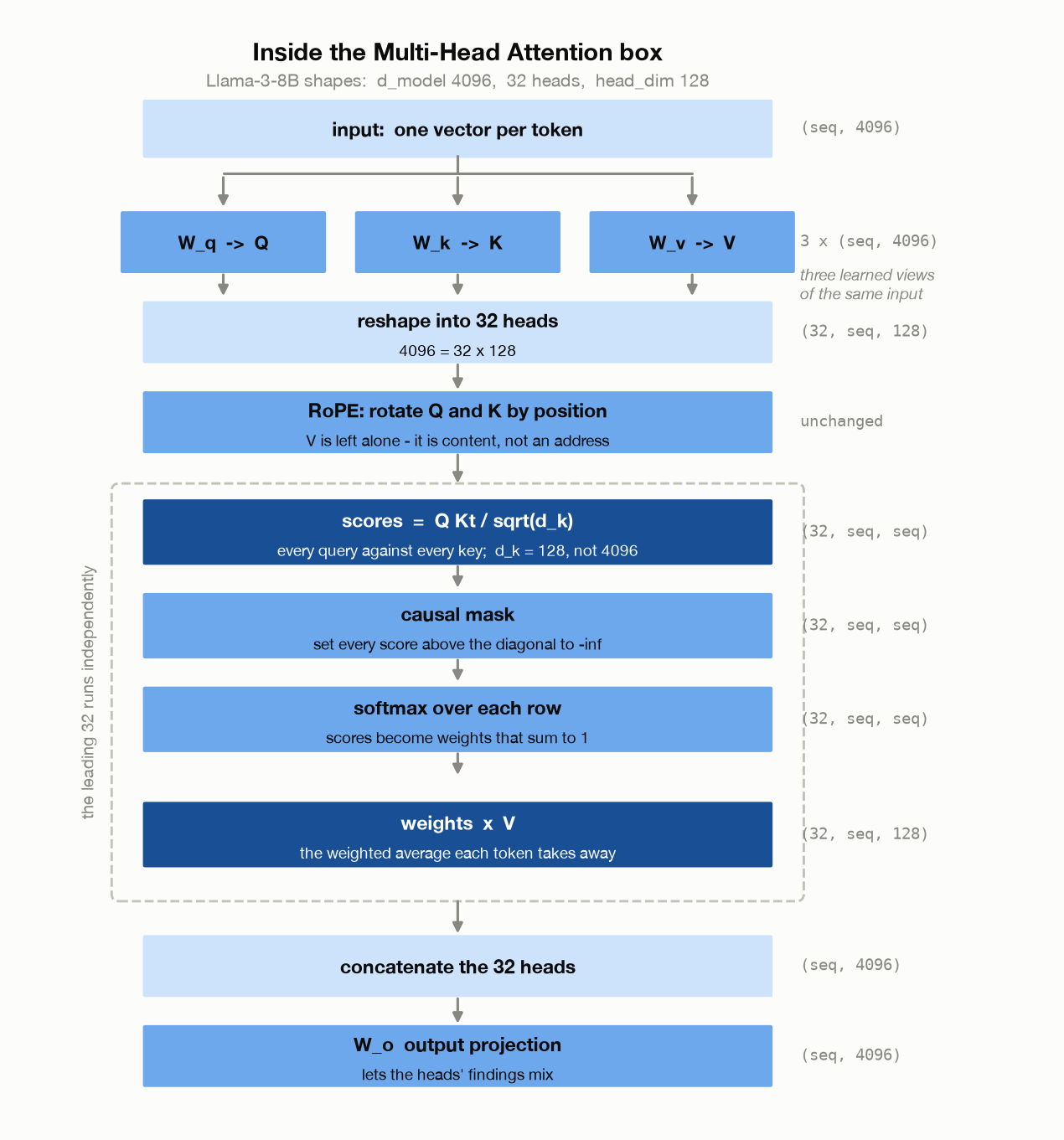
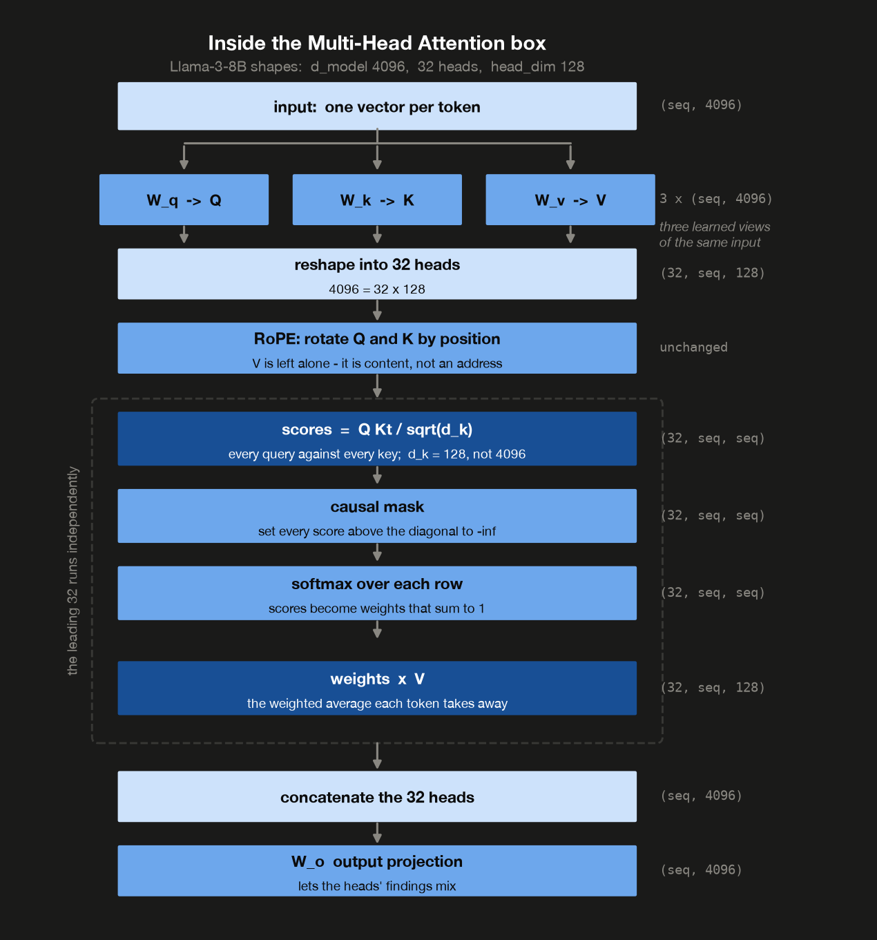
Two steps in it are worth naming. One input, three projections — $Q$, $K$ and $V$ are three learned views of the same vector, which is what makes self-attention “self.” And RoPE rotates $Q$ and $K$, never $V$ — position belongs in the matching step; $V$ is the content you retrieve once matching is done, so rotating it would corrupt the payload. §14 covers RoPE properly.
The other pieces, in plain English
Token embeddings — a lookup table with one row per token the model knows. Llama-3-8B knows 128,256 of them, and each row is 4,096 numbers long. That row is the model’s representation of the token — nothing else about a word enters the network. At the start it encodes only “which token is this.” Each block edits it toward “which token is this, in this context.” The word bank enters generic and leaves nudged toward riverbank or savings account.
RMSNorm — as a vector passes through dozens of layers, its numbers drift, growing until they overflow or shrinking until they vanish. Normalization rescales the whole vector back to a standard size, like setting every track on a mixing desk to a consistent level. Relative proportions survive; only the overall magnitude is standardized.
\[\text{RMSNorm}(x) = \frac{x}{\sqrt{\tfrac{1}{n}\sum x_i^2}} \cdot g\]where $g$ is a learned per-dimension scale. The original transformer used LayerNorm, which also subtracts the mean first. RMSNorm’s contribution — Zhang & Sennrich, Root Mean Square Layer Normalization (2019) — is a discovery, not an invention: that mean-subtraction turned out not to matter. Dropping it costs no quality and saves a pass over the data; the paper reports 7–64% lower running time depending on the model.
The residual, and what “pre-norm” means
The residual is a real bypass. Each sublayer’s input branches off, skips both the norm and the sublayer, and is added back at the $\oplus$. So a sublayer never computes its output — it computes a correction:
\[x \leftarrow x + \text{Attention}(\text{Norm}(x))\]If a sublayer learns nothing useful, the block degrades to the identity rather than to noise. That unbroken path is also the road the gradient travels back down undiminished, which is what lets you stack 80 of these.
“Pre-norm” describes where the norm sits relative to that bypass. The 2017 original (Vaswani et al., Attention Is All You Need, the paper that introduced the transformer) normalized after adding the residual, putting a norm on the trunk itself, so every layer’s output got rescaled on the way through. Modern decoders moved it to the bypassed side: in the diagram the norm sits between the point where the arrow branches off and the sublayer it feeds, so the skip route goes around the norm as well as around the sublayer. That leaves the residual path unnormalized end to end, which is what lets deep models train stably without the learning-rate warmup gymnastics the original recipe needed. Xiong et al., On Layer Normalization in the Transformer Architecture, traced the difference to the gradients at initialization: large near the output under post-norm, well-behaved under pre-norm.
That leaves one box in the diagram unexplained, and it’s the biggest one.
9. The FFN: where the model knows things
FFN stands for feed-forward network. It processes each token entirely on its own — that’s what “position-wise” means; token 5 has no idea token 6 exists. Next to attention it looks like filler. It isn’t, and three questions get at why: what it’s made of, why it’s there at all, and why the model’s facts end up living inside it.
What it’s made of
Not one matrix — three matrices with an elementwise gate between them. For Llama-3-8B, per block:
1
2
3
4
5
6
  matrix          shape  params                          role
  -------------------------------------------------------------
  W_gate  (4096, 14336)   58.7M     opens or closes each slot
  W_up    (4096, 14336)   58.7M  the content each slot offers
  W_down  (14336, 4096)   58.7M        writes the result back
  total                  176.2M        per block, x 32 blocks
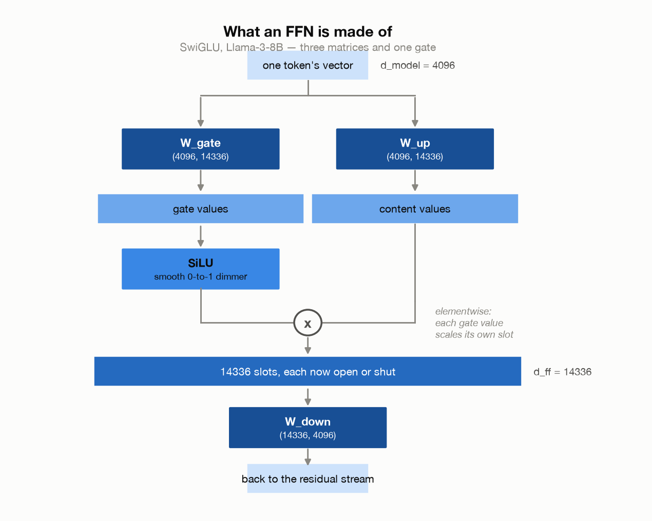
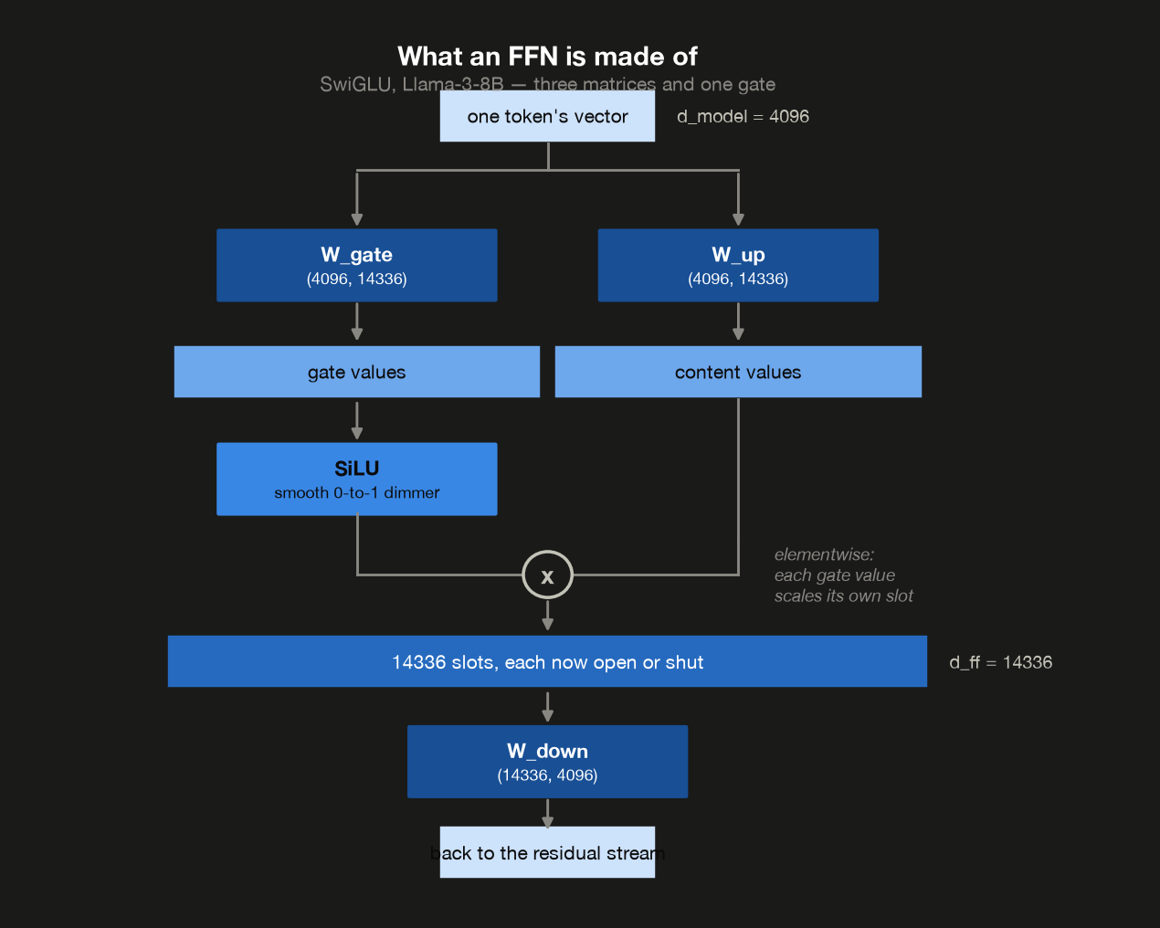
The bars are drawn to scale, so the widening is real: 4096 → 14336 → 4096. Widen, act, narrow.
That gate is SwiGLU, and it’s why there are three matrices rather than two. The original FFN used ReLU — keep positives, zero the negatives — one fixed rule applied to everything, with a single up-projection. SwiGLU replaces the rule with something learned:
\[\text{SwiGLU}(x) = W_{\text{down}}\big(\,\text{SiLU}(W_{\text{gate}}\,x) \;\odot\; W_{\text{up}}\,x\,\big)\]Two up-projections run in parallel. One produces content; the other is squashed by a smooth S-curve (SiLU) into a set of dimmers, and the two are multiplied element by element. The network learns, per feature and per input, how much signal to let through — a dimmer it controls rather than a hard on/off switch. The third matrix is paid for by shrinking the expansion from $4d$ to about $\tfrac{8}{3}d$. That’s how $d_{ff}$ ends up at 14,336 rather than a rounder 16,384.
The paper introducing SwiGLU — Shazeer, GLU Variants Improve Transformer (2020) — is refreshingly candid about this. It tested a family of gated variants, found they worked better, offered no theory, and closed with: “We offer no explanation as to why these architectures seem to work; we attribute their success, as all else, to divine benevolence.” Much of a modern transformer is there because it measured better, not because someone derived it.
Why more than one matrix at all? Because two stacked matrices with nothing between them are one matrix:
Multiply the two matrices together first, then apply the product. If that gives the same answer, the pair was never doing more than a single matrix could:
1
2
3
4
5
    two steps:  (x @ W_up) @ W_down  -11.776383  ...
    one matrix: x @ (W_up @ W_down)  -11.776383  ...

  largest disagreement               3.94e-13
  shape of that single matrix        (64, 64)
Identical. Without a nonlinearity you could pre-multiply $W_{\text{up}}$ and $W_{\text{down}}$ into a single $4096 \times 4096$ matrix and all that widening would buy exactly nothing. The nonlinearity is the only thing stopping them from collapsing into one, which tells you where the work is actually being done.
Why an FFN is needed at all
Because attention can only average. A softmax guarantees two things: the weights are never negative, and they sum to 1. Every output is therefore a blend of the value rows, and a blend of things can never be anything but a mixture of those things.
1
2
3
4
5
6
7
# single head here, so d_k == d_model
w = torch.softmax(q @ k.T / math.sqrt(d_model), dim=-1)
attn = w @ v

(w >= 0).all()                          # every weight non-negative
w.sum(-1)                               # every row sums to 1
torch.allclose(w @ (2 * v), 2 * attn)   # exactly linear in V
1
2
3
4
  softmax weights are all >= 0       yes
  each row of weights sums to        1.0000
  so every output is a blend of V's rows yes
  attn(2V) == 2 x attn(V)            yes
So the output can never leave the range of the values it was handed. And with the weights held fixed, attention is linear in $V$ — that last row is the test, and it comes back in a moment.
The limitation is a real one. Attention can bring “this is a plural noun” and “this sentence is about France” into the same vector, but it cannot compute anything from them. Averaging two facts doesn’t produce a conclusion. “If A and B are both present, then C” is not something a weighted average can express — no matter how many attention layers you stack.
The FFN is the only place in the block where a token’s own features get transformed nonlinearly. The simplest test of the difference:
The doubling test. A linear function must obey $f(2x) = 2f(x)$: feed it twice the input and you get exactly twice the output. That’s what “linear” means.
Run it on both:
1
2
3
4
5
def ffn(t):
    return F.silu(t @ w_up) @ w_down

ffn(2 * x)   # what the function actually returns for a doubled input
2 * ffn(x)   # what a linear function would have returned
1
2
3
4
  function                    f(2x)  2 x f(x)  off by  linear?
  --------------------------------------------------------------
  attention (weights fixed)  23.542    23.542    0.0%      yes
  FFN                        14.641    13.375   21.0%       no
The first two columns are the two things being compared, each summarised by its vector length: what the function actually returns for a doubled input, versus what doubling its output would have given. Attention matches exactly. The FFN doesn’t — so it is not a linear function.
The off by column isn’t something you can derive from the two beside it. It’s the length of the difference between those two output vectors, relative to the linear prediction — $\lVert f(2x) - 2f(x) \rVert / \lVert 2f(x) \rVert$. That’s larger than the 9% gap between the two lengths, because the two outputs don’t merely differ in size: they point in different directions. A linear function couldn’t do that either.
Easier to hold onto with a single number from the output:
1
2
3
    ffn(x) gives                     -0.1197
    2 x that = what linear predicts  -0.2394
    ffn(2x) actually gives           -0.3333
Double the input and a linear function would have moved that number to $-0.2394$. The FFN returns $-0.3333$ instead. It responds to how much signal arrives, not merely in proportion to it. That’s the freedom attention doesn’t have.
Attention decides what to look at; the FFN decides what it means. A meeting where everyone shares information, then the work you actually do with what you heard.
Why knowledge ends up there
The FFN’s shape is a lookup table, the reading developed in Geva et al., Transformer Feed-Forward Layers Are Key-Value Memories (2021). Write it out one slot at a time:
\[\text{FFN}(x) = \sum_{i=1}^{d_{ff}} \underbrace{a_i(x)}_{\text{did slot } i \text{ match?}} \cdot \underbrace{W_{\text{down}}[i]}_{\text{what slot } i \text{ says}}\]where $a_i(x)$ is the activation of the $i$-th middle neuron. Each of the 14,336 middle dimensions is one memory slot with three parts:
| Piece | Role |
|---|---|
| column $i$ of $W_{\text{up}}$ | the pattern slot $i$ looks for |
| $a_i$, its activation | how strongly this token matched it |
| row $i$ of $W_{\text{down}}$ | the content slot $i$ adds if it matched |
Match against stored patterns, then add up the content of whatever matched, weighted by match strength. That’s the same soft-lookup shape as attention itself — except attention looks up other tokens, while the FFN looks up stored weights.
The ordinary matmul and the slot-by-slot sum should be the same thing. Same check as before: take one token’s output and compute it both ways.
1
2
3
acts = F.silu(x @ w_up)                          # one score per slot
from_matmul = (acts @ w_down)[row]               # what the model runs
by_hand = sum(acts[row, i] * w_down[i] for i in range(d_ff))   # slot by slot
1
2
3
4
    from the matmul                  -0.2740  +0.1003  +0.0076  -0.1433
    from the slot-by-slot sum        -0.2740  +0.1003  +0.0076  -0.1433

  largest disagreement, all 64       8.941e-08
So “the model knows Paris is in France” has a concrete home: some slot whose up-projection fires on the Eiffel Tower is in, whose down-projection nudges the output toward Paris. Llama-3-8B has 14,336 slots per layer across 32 layers — 458,752 of them. This isn’t only a metaphor: the ROME and MEMIT lines of work locate specific factual associations in specific FFN weights and edit them, changing what a model believes by writing to a handful of numbers.
The real picture is less tidy than that, in two ways. Slots aren’t cleanly one-fact-each — facts spread across many, and a slot participates in many facts. And with the random weights measured above, most slots respond to anything; trained FFNs are far sparser.
Who gets the parameters?
Counting attention against FFN in a single block, across three real models:
1
2
3
4
5
  block shape                  attention params  FFN params  FFN share
  ----------------------------------------------------------------------
  GPT-2 style (MHA, ReLU FFN)             10.2M       20.5M        67%
  Llama-3-8B (GQA, SwiGLU)                41.9M      176.2M        81%
  Llama-3-70B (GQA, SwiGLU)              151.0M      704.6M        82%
Attention gets the name and the diagrams, but it’s the minority of the weights. The classic two-thirds figure comes from the original shapes — attention $4d^2$, FFN $2 \cdot d \cdot 4d = 8d^2$. Modern decoders push further from both ends: GQA shrinks $K$/$V$ while SwiGLU adds a third FFN matrix.
That’s the parameter-count version of the same point: routing lives in attention, knowledge lives in the FFN. If the FFN is the model’s memory, it needs to be big. It’s also why LoRA on attention alone underperforms, and why Mixture-of-Experts replaces the FFN — both taken up later in this series (MoE in post 5, LoRA in post 6).
10. The implementation, in five lines
1
2
3
4
5
6
7
8
9
10
11
12
13
14
def scaled_dot_product_attention(q, k, v, *, causal=False, scale=None):
    d_k = q.shape[-1]
    scale = scale if scale is not None else 1.0 / math.sqrt(d_k)

    scores = (q @ k.transpose(-2, -1)) * scale  # (..., seq_q, seq_k)

    if causal:
        seq_q, seq_k = scores.shape[-2], scores.shape[-1]
        # True above the diagonal = "this key is in the future" = forbidden.
        mask = torch.ones(seq_q, seq_k, dtype=torch.bool, device=scores.device).triu(1)
        scores = scores.masked_fill(mask, float("-inf"))

    weights = torch.softmax(scores, dim=-1)
    return weights @ v, weights
Shapes are (..., seq, head_dim) — the leading dimensions carry batch and heads, since multi-head attention is this same function applied in parallel. I return the weights alongside the output because they’re exactly what an optimized kernel throws away, and they’re the thing worth looking at.
Checking it against PyTorch’s fused F.scaled_dot_product_attention:
1
2
  max |ours - torch|  (causal=False) 5.364e-07
  max |ours - torch|  (causal=True)  4.768e-07
Agreement to 5e-07 in float32 — floating-point reassociation noise, not an algorithmic difference. Worth internalizing early, because it’s the same fact that makes Flash Attention work: a fast kernel is an optimization, not an approximation. Post 3 returns to this.
11. Why divide by sqrt(d_k)?
The formula back in §3 divides the scores by $\sqrt{d_k}$ before the softmax sees them, and that constant looks like something someone tuned by trial. It isn’t. It’s the one choice that keeps attention behaving the same way no matter how wide you make a head — and getting there takes four small steps, none of which require anything you don’t already have.
One word first. The raw scores going into a softmax — one per key, before any normalizing — are called logits. They’re unbounded, they can be negative, and on their own they mean nothing.
Step 1: a softmax only ever sees gaps
Take the smallest case that shows anything: two keys, with logits $0$ and $g$. The weight landing on the larger one is
\[\frac{e^{g}}{e^{0} + e^{g}} = \frac{1}{1 + e^{-g}}\]Some numbers, since everything below depends on them:
1
2
3
4
5
6
7
  gap g  weight on lower  weight on higher
  ------------------------------------------
  1            0.2689414         0.7310586
  2            0.1192029         0.8807971
  4            0.0179862         0.9820138
  8            0.0003354         0.9996646
  16           0.0000001         0.9999999
Two things follow. The size of those gaps decides everything else: gaps near 1 give a real blend, gaps past about 8 give a winner that takes nearly all of it. And only differences matter, since adding a constant to both logits multiplies the top and bottom of the fraction by the same $e^c$, which cancels:
1
2
3
  softmax([0, 4])                    0.0179862, 0.9820138
  softmax([100, 104])                0.0179862, 0.9820138
  identical                          yes
So asking whether a head will average or pick is the same as asking how far apart its logits are.
Step 2: the size of the gaps is what “temperature” means
Temperature is the standard dial on a softmax, written
\[\text{softmax}(z / T)\]where $z$ are the logits and $T > 0$ is the temperature. Dividing every logit by $T$ divides every gap by $T$ as well, so Step 1 already tells you what it does. A large $T$ shrinks the gaps and flattens the weights toward even, which is called hot; a small $T$ stretches them and sharpens toward one winner, which is called cold. It’s the same dial you set when sampling text from a model.
What matters here is what happens if you never touch the dial. Leaving it alone still sets a temperature, namely $T = 1$, so whatever spread the logits happen to have becomes the temperature you get. Any decision that changes how far apart the logits sit is therefore also a decision about temperature, whether it was meant that way or not.
Head width is one of those decisions.
Step 3: how far apart attention’s logits actually sit
Two terms first, in case they’re rusty. The standard deviation of a set of numbers is their typical distance from the average, which is a reasonable way of saying how big the gaps between them are. The variance is that squared, and it has the property this argument needs: for independent quantities, variances add.
Now take one query $q$ and one key $k$, each $d_k$ numbers long, and assume what holds at initialization: their components are independent of each other, average 0, and have variance 1. The logit is their dot product:
\[q \cdot k = \sum_{i=1}^{d_k} q_i k_i\]Build it up from one term. A single product $q_i k_i$ averages 0, since both factors average 0 and are independent. Its variance is
\[\mathbb{E}[q_i^2 k_i^2] = \mathbb{E}[q_i^2]\,\mathbb{E}[k_i^2] = 1 \times 1 = 1\]That’s one term. The dot product is $d_k$ of them, they’re independent, and variances add, so the variance is $d_k$ and the standard deviation is its square root:
\[\operatorname{Var}(q \cdot k) = d_k \qquad\Longrightarrow\qquad \operatorname{std}(q \cdot k) = \sqrt{d_k}\]So the logits spread over a range of roughly $\pm\sqrt{d_k}$, and head width alone decides how wide that is. At $d_k = 64$ the spread is about 8, and at $d_k = 1024$ about 32, both far down the Step 1 table where a softmax has stopped blending and started picking. Nobody chose that behaviour; it arrived with the head width.
Step 4: so divide by the spread
Dividing every logit by $\sqrt{d_k}$ sets $T = \sqrt{d_k}$ in Step 2, and by Step 3 that is the standard deviation of the logits. Divide a set of numbers by their own standard deviation and they come out with standard deviation 1, whatever they started at. The temperature no longer depends on $d_k$, and head width goes back to being a free choice.
That’s why it’s a square root and not $d_k$ or $\log d_k$: the square root is the function that cancels the spread the dot product actually produces.
The receipt
Now measure it, since Step 3 rested on an assumption about the numbers being independent and unit-variance. Sample random queries and keys at several $d_k$, and report two diagnostics: the average largest weight, where 1.0 is fully one-hot, and the entropy, the same spread measure from §4, written $H$ in the table below. There, 0.0 means all the weight sits on one key and $\ln 8 = 2.08$ means it’s shared evenly across our 8 keys.
1
2
3
4
5
6
7
  d_k   logit std  max w unscaled  H unscaled  max w scaled  H scaled
  ---------------------------------------------------------------------
  4        1.9642          0.5222      1.2986        0.3401    1.7548
  16       3.9493          0.7428      0.6825        0.3523    1.7350
  64       7.9399          0.8738      0.3223        0.3506    1.7407
  256     15.9159          0.9326      0.1691        0.3533    1.7318
  1024    32.4533          0.9735      0.0674        0.3701    1.7103
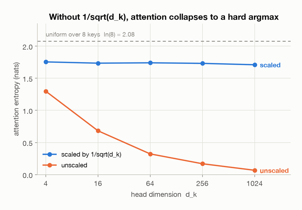
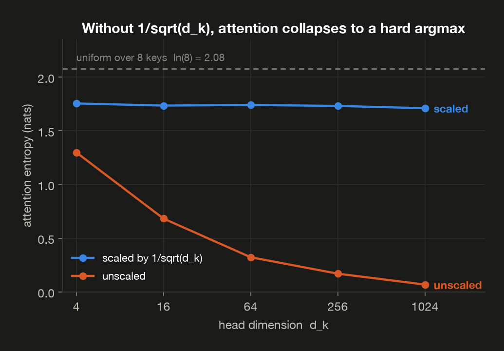
Read the logit std column against Step 3’s prediction: 1.96, 3.95, 7.94, 15.92, 32.45, where $\sqrt{d_k}$ says 2, 4, 8, 16, 32. Close enough that the assumption holds up on real samples.
Then the consequence, which is Step 1 playing out. Unscaled, entropy collapses from 1.30 nats to 0.067; at $d_k = 1024$ the average largest weight is 0.97, so attention has stopped averaging and turned into a hard argmax. Scaled, entropy holds at ~1.74 across a 256× range of $d_k$. The flat blue line is the case for the constant.
Why 1.74 and not the uniform 2.08? Scaling leaves the logits with a standard deviation of 1 rather than 0, so the weights still express preferences: about 0.35 on the favourite, by the max w scaled column. That’s what you want. A head that weighted all eight keys equally would be no more useful than one that picked a single key, and the constant keeps it between those two at any width.
Why saturation breaks training
Two reasons, and the second is the one that does the damage:
- It stops being attention. A near-one-hot distribution ignores all but one token, so the mechanism built to blend information is no longer blending anything.
- The gradient vanishes. Training works by asking, of every number in the model, “if I nudge this up a little, how much does the output change?”, and it only acts where the answer isn’t zero. When the weights already read 0.9999999 and 0.0000001, nudging a logit barely moves them. The answer comes back as zero, which looks exactly like a number that is already correct.
The exact statement behind point 2 uses the softmax’s Jacobian, the matrix holding every one of those “how much does this move that” pairs. It works out to $\operatorname{diag}(p) - pp^\top$. As $p$ approaches one-hot, with one entry at 1 and the rest at 0, every entry of that matrix goes to 0 as well. No gradient reaches $Q$ or $K$, so the model never learns what to attend to.
That second point is the real argument. $1/\sqrt{d_k}$ isn’t about overflow; softmax handles large logits fine by subtracting the row max before exponentiating. It’s there to keep the softmax in a range where a gradient still exists, whatever width you make the heads.
12. Causal masking
§3 introduced the mask $M$. Here is what it does to the weights:
1
2
3
4
5
6
7
        key0    key1    key2    key3    key4    key5
  q0    1.000    0.000    0.000    0.000    0.000    0.000
  q1    0.180    0.820    0.000    0.000    0.000    0.000
  q2    0.366    0.477    0.157    0.000    0.000    0.000
  q3    0.717    0.176    0.072    0.035    0.000    0.000
  q4    0.238    0.015    0.342    0.345    0.060    0.000
  q5    0.126    0.348    0.240    0.160    0.040    0.086
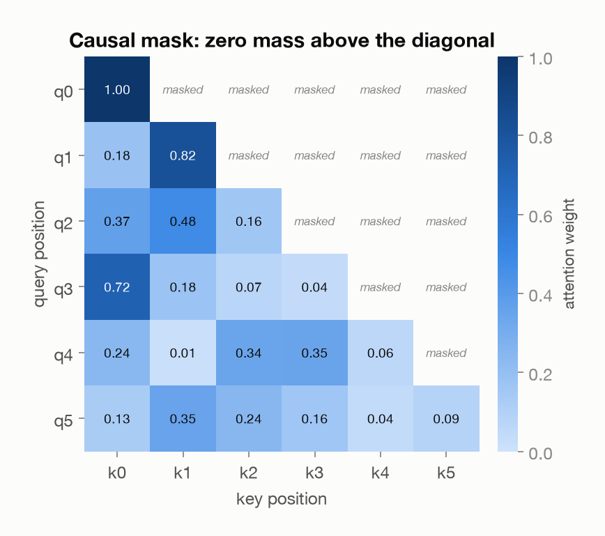
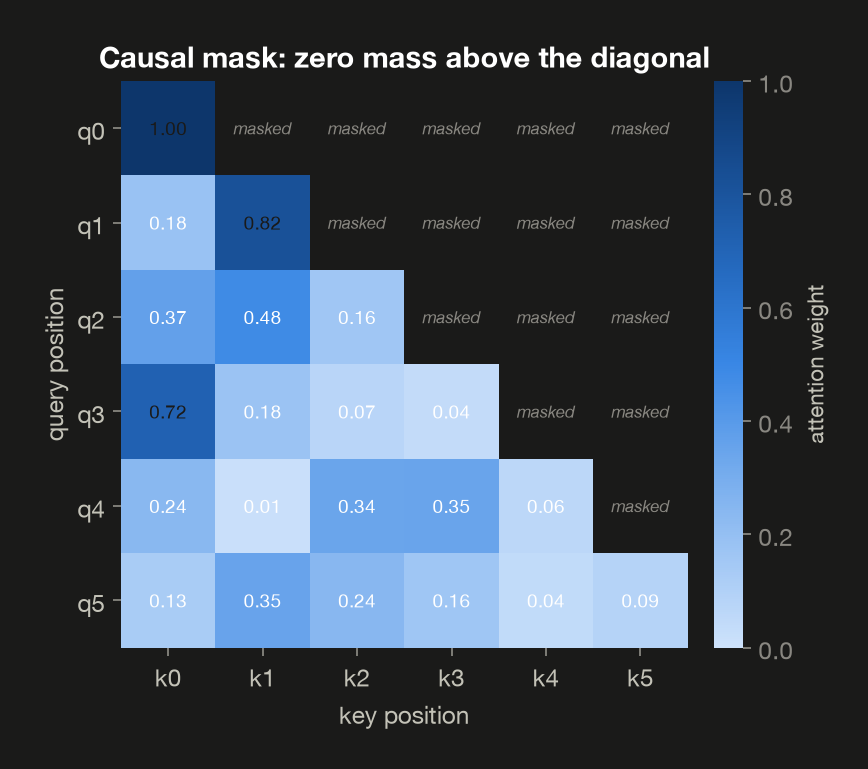
Note row q0: weight exactly 1.000 on itself. The first token has nothing else to attend to, so a softmax over a single unmasked score returns 1.
This one matrix is why the same architecture serves both BERT (unmasked, good for understanding) and GPT (masked, good for generation).
13. How this becomes learning, and becomes writing
Everything so far has described what happens to one token’s vector. That leaves the question this post opened with only half answered: how does a pile of per-token machinery learn anything, or write a sentence?
The answer is that it doesn’t process one token. A forward pass takes the whole sequence at once, and every position produces its own guess at what comes next — position 1 guesses what follows “The”, position 2 guesses what follows “The cat”, and so on. One pass, one guess per position.
Do those guesses feed into each other? No, though the picture invites you to think so. Position 2 sees position 1’s input token, not position 1’s guess. The guesses are all produced together at the very end, by the final layer, and there is no path from one position’s guess to another position’s anything.
The related half of that is checkable, so here it is. Run the model on a five-token sequence, then change one input token and run it again. Every position outputs a score for each word in the vocabulary; the question is whose scores move.
1
2
3
4
5
6
a = torch.tensor([[5, 9, 12, 3, 7]])
b = a.clone()
b[0, 2] = 41                       # swap position 3's token, leave the rest

la, lb = model(a), model(b)        # scores for every word, at every position
(la[0, i] - lb[0, i]).abs().max()  # how far position i's scores moved
1
2
3
4
5
6
7
8
9
10
  first run,  token ids              [5, 9, 12, 3, 7]
  second run, token ids              [5, 9, 41, 3, 7]

  position  its input token  max change in its scores  moved?
  -------------------------------------------------------------
  1                       5                  0.00e+00      no
  2                       9                  0.00e+00      no
  3                12 -> 41                  2.29e+00     yes
  4                       3                  3.14e-01     yes
  5                       7                  1.76e-01     yes
Read it in two halves.
Positions 1 and 2 didn’t budge — 0.00e+00, not close but identical. They were computed from tokens 1–2 and cannot see position 3 at all. That’s the causal mask, showing up as a zero.
Positions 4 and 5 are the interesting ones. Their own input tokens never changed — still 3 and 7 — yet their scores moved anyway, because they attend back to position 3 and it changed underneath them. Information flows forward only, and here you can watch it arrive. The effect fades with distance too: one altered token matters less among four inputs than among three.
So each prediction is a function of the input tokens up to it, and nothing else.
So during training, every position is conditioned on the real text, never on what the model came up with. If position 1 wrongly guessed “dog”, position 2 is still working from the actual “cat” that was in the document. That convention has a name: teacher forcing.
It’s also what lets training be parallel, which is worth pinning down since this post leans on the word repeatedly. It means one specific thing: every position in a document is computed in the same forward pass, at the same time, rather than one after another.
That only works because every position’s input is known before the pass begins. Consider the alternative. If position 2’s input were position 1’s prediction, position 2 couldn’t start until position 1 had finished, position 3 couldn’t start until position 2 had finished, and training on a 4,000-token document would become a chain of 4,000 dependent trips through all 32 blocks. That is the shape generation is stuck with, and the reason generation is slow. Teacher forcing breaks the chain by handing each position the document’s own token instead, and those are all sitting in the file before training starts. Nothing waits for anything, so the whole document goes through together.
Teacher forcing is only half of what makes that legal, though. It supplies all the inputs up front, while the causal mask stops a position from simply reading the answer sitting next to it once they’re all present together. That half comes just below the diagram.
Generation is the one place a guess does feed forward, and only because you explicitly append it and run the whole thing again. That’s the orange arrow in the diagram, and it’s a real difference between the two jobs: the model trains on flawless prefixes and then has to run on prefixes it wrote itself, mistakes included. That mismatch has a name too, exposure bias, and it’s what teacher forcing costs you in exchange for the speed.
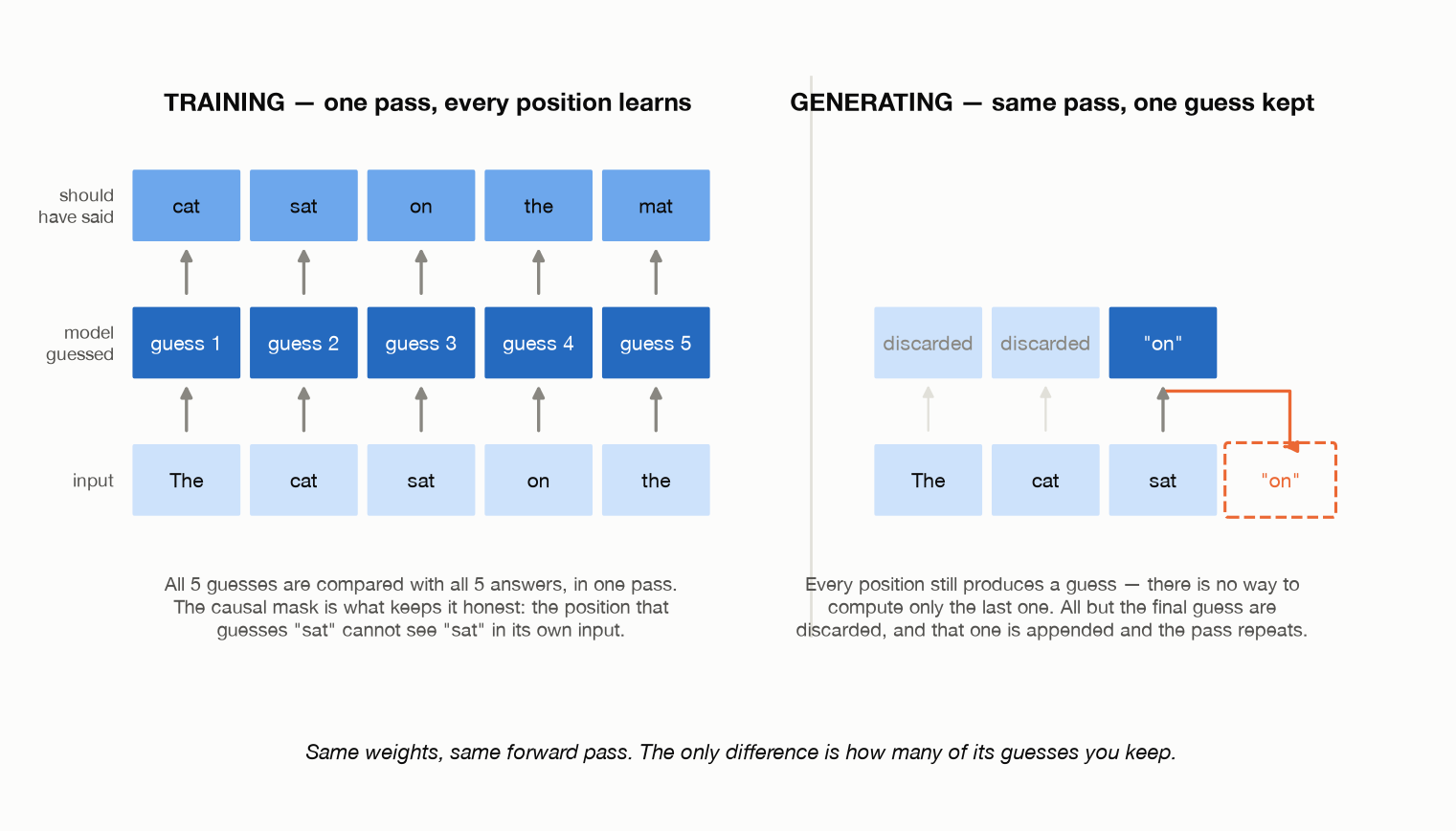
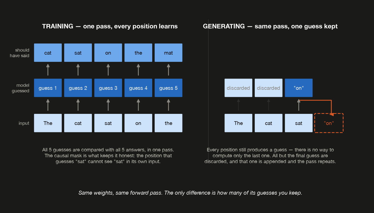
Training grades all of them. You already know what came next — it’s the very next token in the text — so a single pass over a 5-token sentence gives you 5 graded predictions, and over a 4,000-token document, 4,000 of them. The model nudges its weights to make the right answers likelier, and repeats a few trillion tokens’ worth.
This is where the causal mask earns its keep, and it’s the half of the deal left owing above. Position 2 is being asked to guess “sat” while “sat” is sitting right there in the input, two boxes along. The mask is what makes that a real question rather than a copying exercise. Teacher forcing puts all 4,000 tokens in front of the model at once; the mask keeps that from being cheating. You need both to train in one pass.
Generating runs exactly the same pass and throws almost all of it away. You feed in what exists, every position dutifully produces a guess, and you keep only the last one — the others are answers to questions you already know. That kept token gets appended, and the whole thing runs again, one token longer.
The same picture, at the level of the architecture
That diagram shows what each position produces. Here’s where in the model it happens — the stack from §1, doing both jobs:
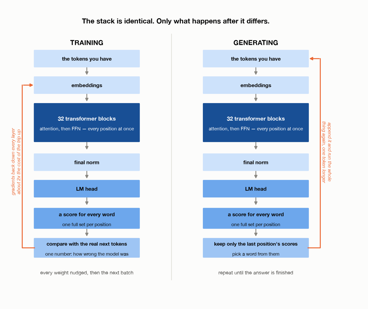
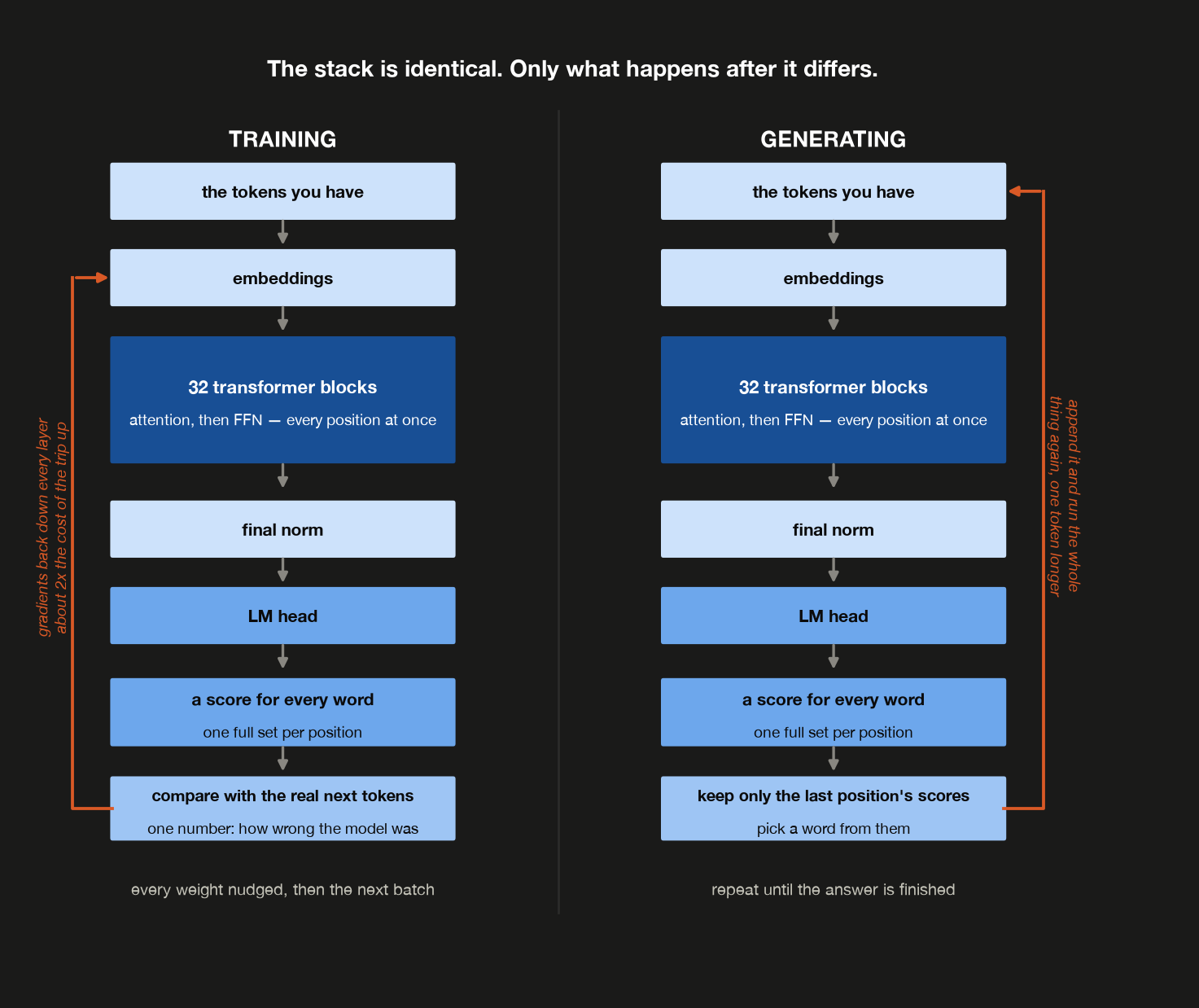
Read down the middle of either column and it’s the same path, box for box: tokens, embeddings, 32 blocks, a final norm, the LM head, and out the bottom a score for every word in the vocabulary — one full set per position, which is the parallelism from the previous diagram, seen from the side.
The difference is entirely in what happens at the bottom.
Training compares all those scores against the real next tokens and boils the result down to one number: how wrong the model was.
Both halves of that sentence are load-bearing. The comparison is possible because the right answer is free — it’s the next token in the document, so a 4,000-token passage arrives with 4,000 labels already attached. The one number is required because a gradient answers “how does this single quantity change if I nudge this weight,” and a forward pass leaves you holding one score per word per position. Those get averaged into a single loss precisely so there is something to push down.
One thing training does not do, though it’s the natural guess: it never picks predicted tokens and compares them to the real ones. Picking means taking the highest score, and that operation has no useful derivative — nudge a weight slightly and the winner doesn’t change, so the gradient is zero almost everywhere and nothing could learn. Instead the model keeps the full distribution and is scored on a softer question: how much probability did you put on the token that actually came next? That answer moves smoothly, so it still gives a direction to travel even when the top guess is wrong. Then comes the part that has no counterpart on the right — the return trip. That error is walked back down through every layer, working out how each individual weight contributed to it, and every weight is nudged. That backward journey is where the extra cost from §6 comes from: roughly twice the forward pass, which is what turns $2N$ into $6N$.
Generating never goes back. It takes the bottom row, throws away everything except the last position’s scores, picks a word from them, sticks it on the end of the input, and runs the entire stack again — 32 blocks, from the top, for one more token. That loop is why a 500-token answer means 500 trips through the whole model.
The return trip, in two matrix multiplies
§6 priced that backward journey at roughly twice the forward pass. Here’s where the factor of two comes from, on a single linear layer — which is what each of the four projections is.
Forward, the layer computes
\[Y = XW \qquad (n, d_{in}) \times (d_{in}, d_{out}) \;\to\; (n, d_{out})\]Coming back, it is handed exactly one thing: $dY$, the gradient of the loss with respect to its own output, shape $(n, d_{out})$. From that single tensor it forms two products:
\[dW = X^\top \, dY \qquad (d_{in}, n) \times (n, d_{out}) \;\to\; (d_{in}, d_{out})\] \[dX = dY \, W^\top \qquad (n, d_{out}) \times (d_{out}, d_{in}) \;\to\; (n, d_{in})\]Check the shapes that fall out. $dW$ comes out exactly the shape of $W$ — one number per weight, which is what the optimizer later consumes. $dX$ comes out exactly the shape of $X$ — one number per input element.
That second one is the message. A layer’s input is the previous layer’s output, $X^{(\ell)} = Y^{(\ell-1)}$, so differentiating the loss with respect to that one tensor produces a single object wearing two names:
\[dX^{(\ell)} \;=\; dY^{(\ell-1)}\]Not an analogy — literally the same tensor. Layer $\ell$ computes $dX$, and that is the $dY$ that layer $\ell-1$ needs before it can form its own two products. The chain runs on that identity, and nothing can be computed out of order because of it.
Now count. All three multiplies contract the same three dimensions, differing only in which axis is summed away, so the $2abc$ rule from §5 prices them identically:
| Operation | FLOPs | |
|---|---|---|
| forward | $XW$ | $2 \, n \, d_{in} \, d_{out}$ |
| backward | $X^\top dY$ | $2 \, n \, d_{in} \, d_{out}$ |
| backward | $dY W^\top$ | $2 \, n \, d_{in} \, d_{out}$ |
One forward, two backward — training costs $3\times$ inference, which is the $2N \to 6N$ from §6, derived rather than asserted.
One more consequence falls out of $dW = X^\top dY$: it needs $X$, the layer’s input from the forward pass. So every layer’s input has to be held in memory from the moment it’s computed until the backward pass comes back for it. That’s the activation memory §6 flags and doesn’t count. Note that $dX = dY W^\top$ needs only $W$ — it’s the weight gradient alone that pins those activations down.
The last two boxes: the final norm and the LM head
Those bottom boxes have appeared in three diagrams now without being opened, and they’re where a vector finally turns back into a word.
The final norm is the same RMSNorm from §8, applied once after the last block. Thirty-two blocks have each added their corrections to the residual stream, and nothing has rescaled it since; this puts the vector back into a predictable range before the last step reads it.
The LM head is one matrix, and conceptually the simplest thing in the model: it takes a token’s 4,096 numbers and produces one score per word in the vocabulary — all 128,256 of them.
That number should look familiar. Back in §8 the model turned a token into a vector by looking up one of 128,256 rows. The LM head is a table of the same shape doing the same job in reverse: instead of fetching one row by its number, it compares your vector against every row and reports how well each one matches. A lookup is just what that comparison collapses to when you hand it a single token id instead of a blended vector, which is why the two feel like one object.
Same shape and a mirrored job, but not the same numbers. In Llama-3-8B these are two separate $128{,}256 \times 4{,}096$ matrices, each trained on its own, and nothing forces the row for cat on the way in to resemble the row for cat on the way out. Sharing them is a design decision called weight tying, and the parameter count below is where that decision shows up.
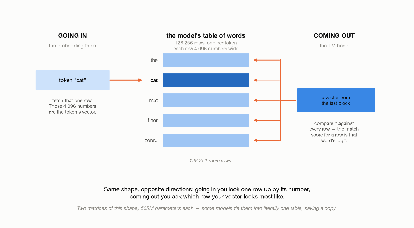
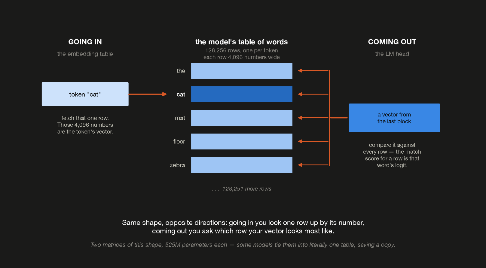
Read left to right, that is the whole model in one line: a word becomes a row, thirty-two blocks edit that row’s numbers using the other words present, and then you ask which row the edited numbers now look most like. Predicting a word is a similarity search over the vocabulary.
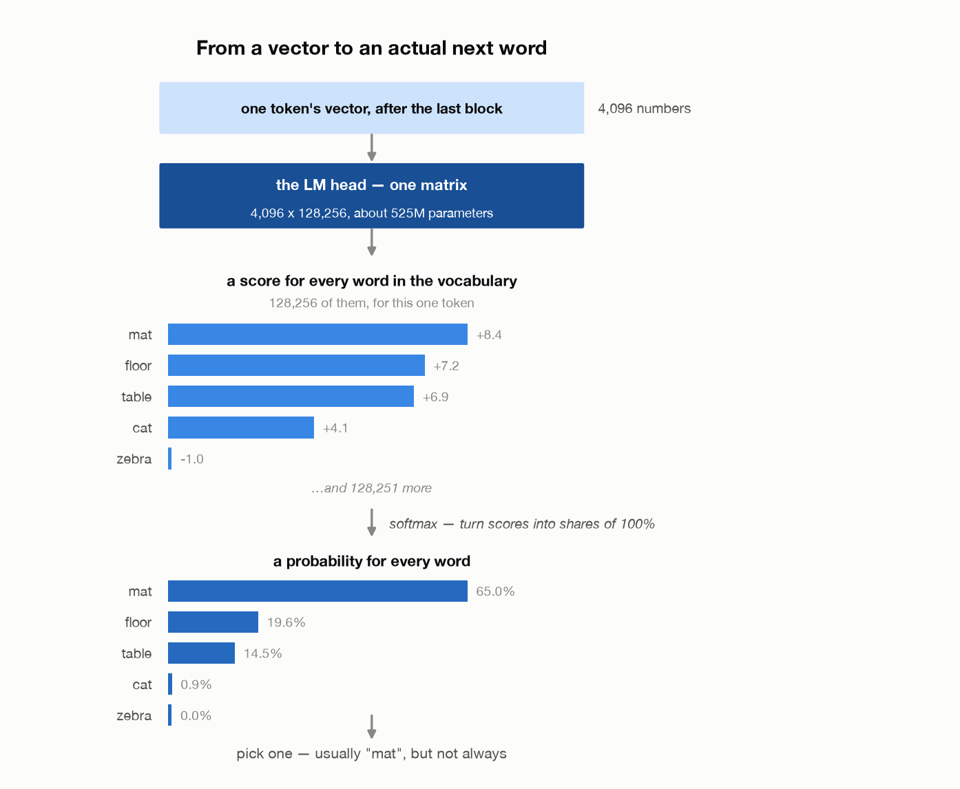
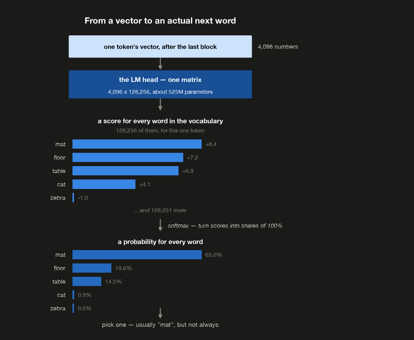
Those raw scores are logits again — the same word as §11, now over the vocabulary rather than over keys, and with the same two properties: unbounded, and meaningful only through their differences. Softmax turns them into shares of 100%, and then a word is drawn from that distribution. Always taking the highest-scoring word makes the model repetitive, so real sampling deliberately keeps some of the randomness. That’s what makes the same prompt give different answers twice.
Two things about this step surprise people.
It’s a huge matrix. It needs one row of 4,096 weights for each of the 128,256 words it scores, so its size is $n_{vocab} \times d_{model} = 128{,}256 \times 4{,}096$ — 525M parameters, which against the model’s 8.03B is 6.5% sitting in a single layer. The embedding table is exactly the same size, for exactly the same reason, so double it: $2 \times 525\text{M} = 1.05\text{B}$, or 13% of the model in two lookup tables, leaving the 32 blocks the other 87%. Since they hold the same kind of thing, some models tie them — one set of weights used in both directions, saving the 525M outright.
You can read which one a model chose off its advertised size:
1
2
3
4
5
6
7
8
9
10
11
  one table (n_vocab x d_model)      525.3M
  one block (attention + FFN)        218.1M
  32 blocks                          6.979B

  arrangement                 tables  total parameters
  ------------------------------------------------------
  untied (separate matrices)       2            8.030B
  tied (one shared matrix)         1            7.505B

  Llama-3-8B is advertised as        8.03B
  so it keeps them                   separate
GPT-2 tied its two, and so do several of the smaller models released since, where 525M is a much larger share of the budget.
Its output is enormous during training. One token’s logits are 128,256 numbers, and the bytes rule turns a count into a size: the loss is computed in fp32, so 4 bytes each, and $128{,}256 \times 4 = 513$ KB. That’s the half a megabyte — one token’s worth of scores.
Half a megabyte is nothing on its own. The trouble is that training scores every position at once, so a 4,096-token sequence holds all of them together:
\[4{,}096 \times 128{,}256 \times 4 \text{ bytes} \;\approx\; 2.1 \text{ GB of logits}\]And that is a memory cost, not a compute one, which is worth separating because the LM head is unremarkable on the compute side. By the $2N$ rule it costs $2 \times 525\text{M} = 1.05$ GFLOP per token against the whole model’s 16.1, or 6.5%. That’s exactly its share of the parameters, since the rule charges every weight alike. Nothing surprising there.
What’s out of proportion is the tensor it leaves lying around. Those 2.1 GB have to stay in memory until the backward pass consumes them, which makes a single layer’s output bigger than every other stored activation in the model put together; §6 measures those at 1.1 GB with checkpointing on. That’s what chunked loss computation is for: split the positions into groups, compute the loss group by group, and never hold the whole tensor at once.
So what actually runs in parallel?
Worth laying out plainly, because “the transformer is parallel” is true of some axes and flatly false of others. The rule underneath is simple: things run in parallel exactly where nothing depends on anything else.
| Across | In parallel? | Why |
|---|---|---|
| the 32 heads | yes | they never touch each other until $W_o$ |
| positions, going forward | yes | each prediction depends on input tokens, never on another prediction |
| positions, going backward | yes | one backward sweep produces the gradients for all positions at once |
| the 32 blocks | no | block 2’s input is block 1’s output |
| forward vs backward | no | the backward pass needs the values the forward pass computed |
| tokens you’re generating | no | token 502’s input is token 501’s output, which doesn’t exist yet |
The first three are why training is efficient at all. A 4,000-token document goes through in one forward sweep and one backward sweep, and both of those handle every position simultaneously — you are never looping over tokens.
The last row is the one that costs you. Generation cannot be parallelised over the thing you actually want more of. You can process a 4,000-token prompt in a single pass, because those tokens already exist; you cannot produce a 4,000-token answer in a single pass, because each token has to exist before the next one can be conditioned on it. 4,000 sequential trips through all 32 blocks.
That asymmetry — a prompt read in one pass, an answer written one token at a time — is the single most consequential fact about running these models, and it’s what post 2 is about.
Two more things follow, and they’re the seeds of the next two posts:
- Nothing computes “just the last position”. The machinery is inherently parallel across the sequence; you can’t ask it for one prediction. So generating a 500-token reply means 500 passes, each slightly longer than the last — and each recomputing what the previous one already worked out. That waste is what a KV cache exists to remove.
- Training and generating are the same forward pass, which is why every cost in §5 applies to both. What differs is that training adds a backward pass, and that generating repeats the forward one over and over for a single answer.
14. RoPE: absolute rotation, relative score
Back to the gap from §3: attention has no idea what order the tokens came in. Something must inject position.
The original transformer solved this by adding a position vector to each embedding. §3.5 of Attention Is All You Need builds that vector out of sines and cosines of the position, sized to match $d_{model}$ so the two can be summed. It encodes absolute position, so token 5 gets the vector meaning “5”, and that turns out to be the wrong thing to hand a dot product, for two reasons.
The position gets mixed in with the meaning. The encoding is added straight into the same 4,096 numbers that carry what the token is, and it then falls to $W_q$ and $W_k$ to pull the two apart well enough that the score comes out sensitive to distance. Nothing in the architecture makes that happen. The model has to learn it.
And it has to learn it over and over. Language mostly cares about relative position: “the adjective two tokens back” is the same useful pattern at position 5 and at position 5,000. Under absolute encodings those two arrive as unrelated input patterns, the vector for 5 meeting the vector for 7 in one case and 5,000 meeting 5,002 in the other. One fact about language, learned separately at every offset the training data happened to show it.
Rotary Position Embedding — Su et al., RoFormer: Enhanced Transformer with Rotary Position Embedding (2021) — fixes both by changing where position is applied. Instead of adding it to the vector before the projections, it rotates $Q$ and $K$ afterwards, so position lands in the score itself. Sensitivity to distance is no longer something the model has to learn; the geometry provides it.
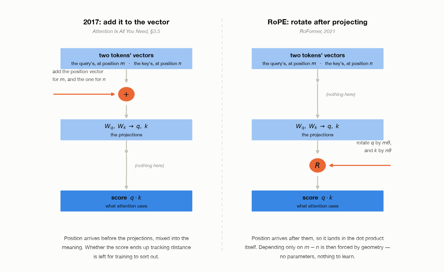
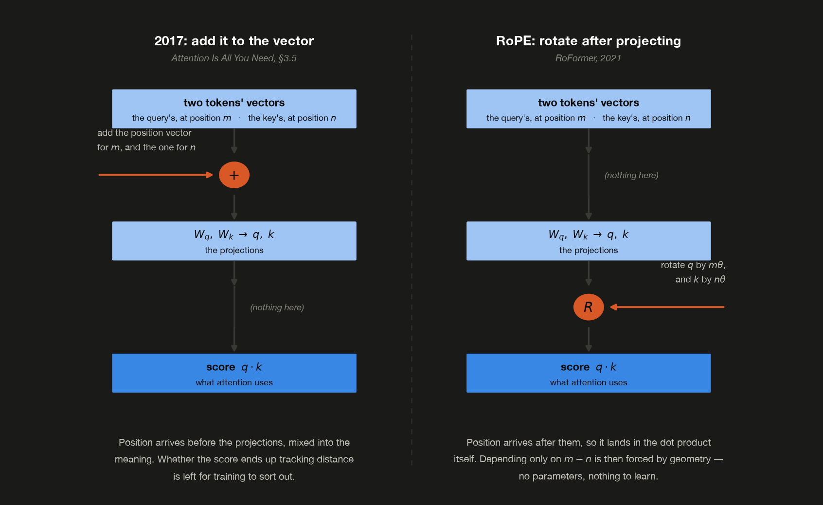
Two tokens are in play throughout, since a score always involves a pair. $m$ is the position of the token doing the looking, whose vector becomes the query $q$, and $n$ is the position of the token being looked at, whose vector becomes the key $k$. If the query sits at 4,093 and the key at 4,096, then $m = 4{,}093$, $n = 4{,}096$, and the gap between them is $m - n = -3$.
Both columns run the same five-stage path, and the only difference is which rung the orange arrow lands on. Anything above the projections is upstream of learning: the model gets vectors with position stirred into them and has to make something of that. Anything below arrives directly in the dot product, where the score is formed.
The rest of this section is why that second placement works at all. It takes four steps, and the first two carry most of the idea.
Step 1: a dot product never sees absolute direction
The score attention computes is $q \cdot k$, and for any two vectors that equals
\[q \cdot k \;=\; \lVert q \rVert \, \lVert k \rVert \cos\alpha\]where $\lVert q \rVert$ is the length of $q$ (its magnitude, the same quantity under either name) and $\alpha$ is the angle between the two. So a dot product depends on exactly three things: the two lengths, and the angle between the vectors.
What it never depends on is which way either vector points on its own. Turn $q$ ninety degrees and turn $k$ ninety degrees the same way, and the score doesn’t budge, since neither length has changed and neither has the angle between them. Absolute orientation is invisible to a dot product; only the relative angle gets in.
That’s the opening to work with. If a score only responds to a difference of angles, then encoding position as an angle should give a score that only responds to a difference of positions.
Step 2: rotate each vector by its own position
Work in two dimensions first, where “rotate” means exactly what it sounds like.
Let $q$ point at angle $\varphi_q$ and $k$ at angle $\varphi_k$, so before position enters, their score is $\lVert q \rVert \lVert k \rVert \cos(\varphi_q - \varphi_k)$. Now place the query at position $m$ and the key at position $n$, and turn each one by its own position times a fixed rate $\theta$:
| angle before | angle after | |
|---|---|---|
| query, at position $m$ | $\varphi_q$ | $\varphi_q + m\theta$ |
| key, at position $n$ | $\varphi_k$ | $\varphi_k + n\theta$ |
Rotating a vector never changes its length, so the lengths in Step 1 are untouched and the only thing that moves is the angle between them:
\[(\varphi_q + m\theta) - (\varphi_k + n\theta) \;=\; (\varphi_q - \varphi_k) \;+\; (m-n)\,\theta\]That line is the mechanism. Two absolute positions went in, and only their difference $m-n$ came out, because the $m\theta$ and $n\theta$ terms subtract. The score is now
\[q_m \cdot k_n \;=\; \lVert q \rVert \lVert k \rVert \cos\!\big((\varphi_q - \varphi_k) + (m-n)\theta\big)\]which comes out the same for a query at 5 reading a key at 8 as for a query at 4,093 reading a key at 4,096, since both are three apart. Written compactly, with $R_m$ meaning “rotate by $m\theta$”:
\[\langle R_m q,\; R_n k \rangle = \langle R_{m-n}\, q,\; k \rangle\]No learned parameters appear anywhere in that derivation. The invariance is a property of rotation itself, not something the model had to be taught.
Step 3: but a head is 128 numbers, not 2
Rotation is a two-dimensional idea, so RoPE cuts a head’s 128 dimensions into 64 independent planes and spins each plane on its own. That costs nothing, because a dot product over 128 numbers is just the sum of the 64 planes’ dot products:
\[q \cdot k \;=\; \sum_{i=1}^{64} \big(q \cdot k\big)\big\vert_{\text{plane } i}\]By Step 2, every term on the right depends only on $m-n$. A sum of things that each depend only on $m-n$ depends only on $m-n$, so the property survives the scale-up.
Step 4: why the planes spin at different speeds
If all 64 planes turned at the same rate $\theta$, the score would come down to $\cos((m-n)\theta)$, and a cosine repeats. Offsets of 3 and of $3 + 2\pi/\theta$ would give identical scores, and the model could not tell “three tokens back” from “three tokens and one full turn back.”
Giving each plane its own rate fixes that, for the same reason a clock has more than one hand. The second hand is precise but comes round every minute; the hour hand is coarse but doesn’t wrap all day; only together do they name a time unambiguously. RoPE’s rates run geometrically from fast to slow. These are the $\theta_i$ in the code below, built on the same base of 10,000 as the 2017 sinusoids:
\[\theta_i = 10{,}000^{-i/d_{head}}, \qquad i = 0, 2, 4, \ldots, 126\]1
2
3
4
5
6
7
plane i theta_i full circle every
-----------------------------------------
0 1 6 positions
32 0.1 63 positions
64 0.01 628 positions
96 0.001 6,283 positions
126 0.000115478 54,410 positions
The fast planes resolve close neighbours sharply and wrap constantly. The slow ones have barely begun to turn by the end of a long context, so they carry coarse, long-range position instead. Read all 64 together and the offset is pinned down exactly.
That table is also where context extension happens. Every method you’ve heard of, position interpolation and NTK-aware scaling and YaRN, is some way of rescaling that column of rates, so rotations learned at 4k still mean something at 128k.
The code
1
2
3
4
5
6
7
8
9
10
11
12
13
14
15
16
def rope_frequencies(head_dim, base=10_000.0):
    i = torch.arange(0, head_dim, 2, dtype=torch.float64)
    return 1.0 / (base ** (i / head_dim))

def rotate_half(x):
    """[x1, x2] -> [-x2, x1]: a 90-degree rotation in each 2D subspace."""
    x1, x2 = x.chunk(2, dim=-1)
    return torch.cat((-x2, x1), dim=-1)

def apply_rope(x, positions, base=10_000.0):
    head_dim = x.shape[-1]
    pos = positions.cpu().to(torch.float64)[:, None]
    angles = torch.cat([pos * rope_frequencies(head_dim, base)] * 2, dim=-1)
    cos = angles.cos().to(torch.float32).to(x.device).to(x.dtype)
    sin = angles.sin().to(torch.float32).to(x.device).to(x.dtype)
    return x * cos + rotate_half(x) * sin
The last line is the only one that looks like sleight of hand. Turning a plane $(x_1, x_2)$ by $\alpha$ gives $(x_1\cos\alpha - x_2\sin\alpha,\; x_1\sin\alpha + x_2\cos\alpha)$ — and that is exactly x * cos + rotate_half(x) * sin, once rotate_half is the map $(x_1, x_2) \to (-x_2, x_1)$. Doing it this way means the code pairs dimension $j$ with dimension $j+64$ rather than with its neighbour $j+1$: the same 64 planes as Step 3, just sliced for cheaper tensor operations, which is where the name rotate_half comes from.
Now the receipt, which tests the claim from Step 2 directly: if the score really depends only on $m-n$, sliding both tokens along the sequence while holding the gap fixed should change nothing.
So take one query vector and one key vector, the same two throughout and never re-drawn, and try them at four different pairs of positions, always three apart:
1
2
3
4
5
6
7
8
  query pos m  key pos n  offset m-n  q_m . k_n
  -----------------------------------------------
  0                    3          -3    -1.1905
  5                    8          -3    -1.1905
  105                108          -3    -1.1905
  4093              4096          -3    -1.1905

  range across absolute positions    1.073e-06
Read a row left to right: put that query at position $m$, put that key at position $n$, rotate each by its own position, take the dot product. The first row is a query at 0 against a key at 3, the last a query at 4,093 against a key at 4,096. Very different places in the sequence, identical gap. (The offset comes out negative because the query sits before the key in these pairs. This is the bare geometry, with no causal mask in play.)
The final column is the answer, and it never moves: $-1.1905$ in all four rows. The line beneath it is that column’s range, largest minus smallest, and at 1.073e-06 that’s floating-point noise rather than a real difference. Position 5 and position 4,093 give the same score to seven digits.
So the model never has to relearn “3 tokens back” for each position in the window. It gets that invariance from geometry, with zero learned parameters, which is the thing the additive scheme was making it work for.
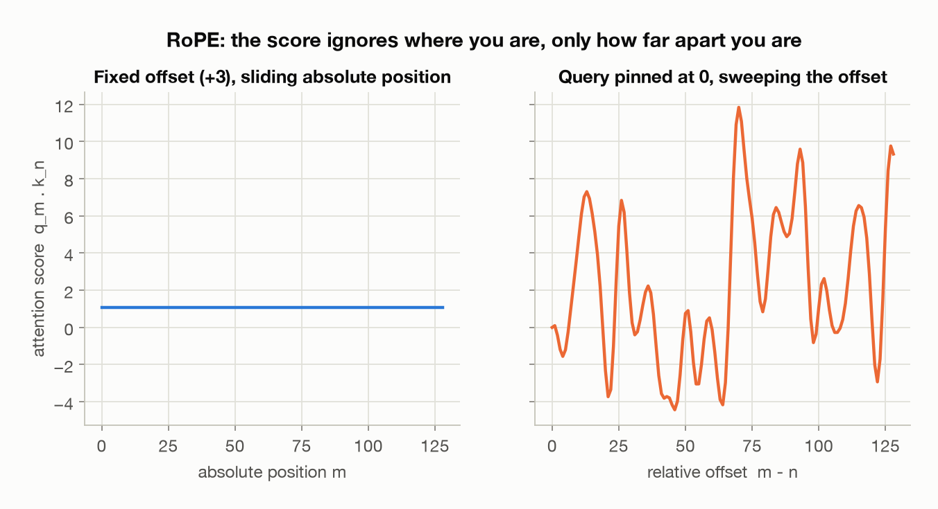
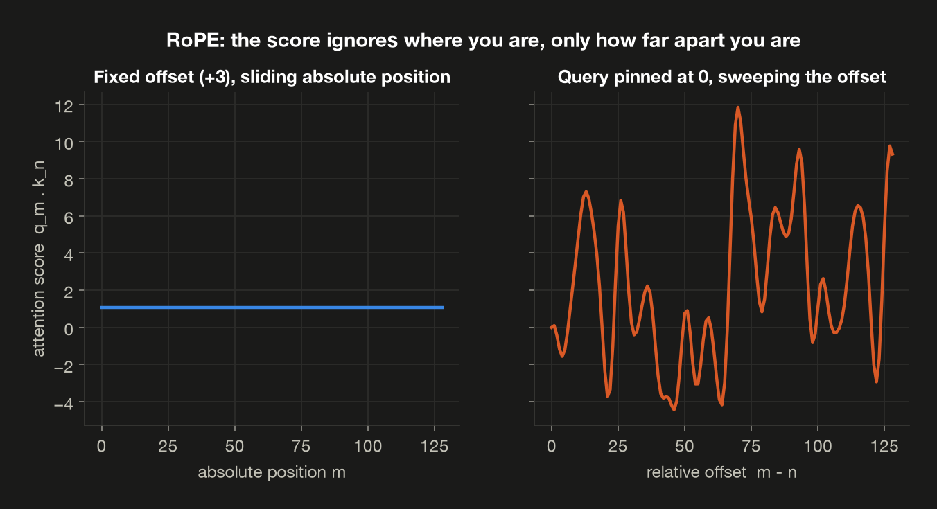
Two panels, same y-axis. Left: slide both vectors along 128 positions, holding the gap at +3 — a flat line. Right: pin the query and sweep the offset — structure everywhere. Flat where you want invariance, expressive where you want sensitivity.
Where a context window actually comes from
That also settles the question §5 left open: what makes a model “128k”?
Not the architecture. Every weight matrix in this post is sized by $d_{model}$, $d_{ff}$ or the vocabulary — not one of them mentions sequence length, so the same weights run on ten tokens or ten million. Older models did have a hard wall, because they learned position: a table with one row per slot, and no row 513 if you trained 512 of them. RoPE has no such wall. The rotation for position 500,000 is a formula, and it computes perfectly well.
What’s left is experience. The model has only ever seen rotations from the range it trained on, and past that edge the angles are unfamiliar and quality falls away. So the advertised window is a claim about where quality was checked, not a limit sitting in the weights. That’s also why it tends to be bought in two stages. Training cost grows with $seq$, so a model does the overwhelming bulk of its training short and cheap, then extends in a brief final phase that rescales the frequency vector until rotations learned at the short length still mean something at the long one. Llama 3 pretrained at 8k; Llama 3.1 stretched the same architecture to 128k.
The number is optimistic in two ways. Models routinely degrade well before their stated limit — “128k” means “doesn’t fall apart,” not “equally sharp throughout.” And inference servers enforce the ceiling for an unrelated reason: the KV cache grows with every token, so serving needs a fixed memory budget per request. That one is post 2.
One consequence worth flagging now: because the rotation happens after the $Q$/$K$ projections, RoPE doesn’t commute with tricks that absorb those projections into neighbouring matrices. That’s the complication DeepSeek’s MLA has to work around, and the planned capstone of this series (post 12) is where it gets picked up.
15. A silent MPS bug that deleted RoPE
While building this demo, the RoPE section printed a score that was identical for every offset. Not wrong-looking — suspiciously perfect.
The angle table needs float64: at position 4096 the fastest frequency has accumulated ~4096 radians, and float32 has about 7 digits for an argument that large. So I moved positions to the CPU and cast in one call — the idiomatic thing to write:
1
pos = positions.to("cpu", torch.float64)     # looks fine. is not.
On an int64 MPS tensor, torch 2.13 reinterprets the bits instead of converting them. The reason that slips through is that PyTorch does guard this path, just not for the dtype a tensor of positions happens to be:
1
2
3
4
5
6
7
i = torch.tensor([105], device='mps')     # int64 — what positions always are
f = torch.tensor([105.0], device='mps')   # float32

i.to('cpu', torch.float64)    # tensor([5.1877e-322])  <- 105's bits read as a float
i.cpu().to(torch.float64)     # tensor([105.])         <- correct
f.to('cpu', torch.float64)    # TypeError: MPS doesn't support float64
i.to('cpu', torch.float32)    # tensor([105.])         <- correct
Ask a float MPS tensor for float64 and you get a loud refusal. Ask an int64 one, which is what a list of positions is, and a number comes back. One dtype away from the exception that would have ended the search immediately.
5.19e-322 is a denormal indistinguishable from zero. Every angle became 0, so cos = 1, sin = 0, and x * 1 + rotate_half(x) * 0 returned x unchanged. RoPE had silently degraded into the identity function — no exception, no warning, just a model with no positional information that would have trained to a mediocre loss and left me blaming hyperparameters.
The fix is to separate the device move from the dtype cast. The general lesson: when a numerical result looks too clean, check it on a second device. LLMR_DEVICE=cpu uv run demo01 takes two seconds and would have caught this immediately.
Sidebar: the probe
“Why is there a $1/\sqrt{d_k}$ in the attention equation?”
A weak answer: “For numerical stability — it keeps the dot products from getting too large.”
Not wrong, but it doesn’t survive a follow-up. Softmax is already robust to large logits: every implementation subtracts the row max first, so [1000, 1001, 1002] and [-2, -1, 0] give identical output. Overflow isn’t the problem being solved.
A stronger answer: “The dot product of two $d_k$-dimensional unit-variance vectors has variance $d_k$, so without the scale the logits grow like $\sqrt{d_k}$ and the softmax sharpens as you widen the heads. Once it saturates toward one-hot, the Jacobian $\operatorname{diag}(p) - pp^\top$ goes to zero and no gradient reaches $Q$ and $K$ — the model can’t learn what to attend to. The scale holds the temperature roughly constant, so head width stays a free architectural choice instead of something that silently changes training dynamics.”
The difference is that the second answer says what breaks, and where.
What’s next
Post 2 takes the same measure-it-yourself approach to the KV cache — the thing that decides what you can actually serve. It times generation with and without one, works out why decode is memory-bandwidth-bound while prefill is compute-bound, and shows why that single distinction explains batching, quantization and speculative decoding at once. Post 3 goes after the $seq \times seq$ score grid from §5, and how Flash Attention gets attention’s answer without ever writing it down.
Both are drafted and will go up shortly.
Appendix: all notation
| Symbol | Means | Llama-3-8B |
|---|---|---|
$n$, seq | tokens in the sequence | varies with input |
| $d_{model}$ | width of a token’s vector | 4096 |
$n_{heads}$, n_heads | number of attention heads | 32 |
| $h$ | index of a single head, $0 \ldots n_{heads}-1$ | — |
| $d_{head}$, $d_k$ | width of one head’s slice | 128 |
| $d_{ff}$ | width of the FFN’s middle layer | 14336 |
| $L$ | blocks stacked | 32 |
| $n_{vocab}$ | vocabulary size — how many distinct tokens exist | 128256 |
| $x$ | the input, one vector per token | $(n, 4096)$ |
| $W_q$ | projection producing $Q$ | $(4096, 4096)$ |
| $W_k$, $W_v$ | projections producing $K$ and $V$ — a quarter as wide, because GQA | $(4096, 1024)$ |
| $Q$ | queries before the head split | $(n, 4096)$ |
| $K$, $V$ | keys and values before the head split | $(n, 1024)$ |
| $Q$ | the same tensor after the head split | $(32, n, 128)$ |
| $K$, $V$ | the same tensors after the split — 8 heads, broadcast back to 32 for the matmul | $(8, n, 128)$ |
| $W_o$ | output projection | $(4096, 4096)$ |
| $\oplus$ | residual addition | — |
| $\odot$ | elementwise multiply (SwiGLU’s gate) | — |
| $R_m$ | RoPE’s rotation for position $m$ | — |
| $\theta_i$ | RoPE’s rotation rate for plane $i$ — how far it turns per position | $10{,}000^{-i/128}$ |
| $\varphi_q$, $\varphi_k$ | the angle a query or key points at, before position is applied | — |
| $\alpha$ | the angle between two vectors, as in $q \cdot k = \lVert q \rVert \lVert k \rVert \cos\alpha$ | — |
| $T$ | softmax temperature — logits are divided by it before the softmax | $\sqrt{d_k}$ in attention |
| FLOP | one floating-point add or multiply; a matmul $(a,b)\times(b,c)$ costs $2abc$ | — |
| MHA | multi-head attention — one key/value head per query head | 32 of each |
| GQA | grouped-query attention — several query heads share one key/value head | 32 query, 8 kv |
$Q$, $K$ and $V$ each get two rows because they have two shapes — full width leaving the projection, regrouped into heads immediately after. Nothing is added or discarded between them ($32 \times 128 = 4096$ for queries, $8 \times 128 = 1024$ for keys and values); papers write $Q$ for both shapes and leave you to infer which is meant.
The right-hand column is Llama-3-8B as it actually is — grouped-query, so $K$ and $V$ are a quarter the width of $Q$ and the block holds 41.9M attention parameters rather than 67.1M. §5 works in the classic multi-head shapes, where all four projections are $(4096, 4096)$, because that is the arrangement the arithmetic is easiest to see in; §14 makes the swap explicit. Both are correct for what they describe — just don’t carry §5’s $4d^2$ over to this model unchanged. Here $W_k$ and $W_v$ are a quarter of that width, 4.2M parameters each instead of 16.8M, which is exactly where 67.1M becomes 41.9M.
Two naming traps, because papers are inconsistent about both:
- $d_k$ almost always means $d_{head}$, not $d_{model}$. Substituting 4096 for 128 makes the whole scaling argument come out wrong.
- Keys and values have separate widths in principle ($d_k$ and $d_v$); the original paper distinguishes them. Every model sets them equal, so this post writes $d_{head}$ for both.
References
- Vaswani et al., Attention Is All You Need (2017) — the scale factor is justified in a footnote in §3.2.1; the post-norm arrangement of §8 is stated in §3.1 as $\text{LayerNorm}(x + \text{Sublayer}(x))$, and the warmup schedule it needed is §5.3.
- Olsson et al., In-context Learning and Induction Heads (2022) — the head specialization §4 mentions: previous-token heads and induction heads, named and traced. Builds on Elhage et al., A Mathematical Framework for Transformer Circuits (2021), where induction heads were first identified.
- Su et al., RoFormer: Enhanced Transformer with Rotary Position Embedding (2021) — the RoPE paper behind §14.
- Chen et al., Extending Context Window of Large Language Models via Position Interpolation (2023).
- Peng et al., YaRN: Efficient Context Window Extension of Large Language Models (2023).
- Zhang & Sennrich, Root Mean Square Layer Normalization (2019) — the RMSNorm paper behind §8; it reports 7–64% lower running time than LayerNorm depending on the model.
- Xiong et al., On Layer Normalization in the Transformer Architecture (2020) — the pre-norm vs post-norm analysis behind §8: post-norm’s gradients are large near the output at initialization, which is why the original recipe needed warmup.
- Shazeer, GLU Variants Improve Transformer (2020) — the SwiGLU paper behind §9; the divine-benevolence line is the last sentence of its §4.
- Geva et al., Transformer Feed-Forward Layers Are Key-Value Memories (2021) — where the lookup-table reading comes from.
- Meng et al., Locating and Editing Factual Associations in GPT (2022) — ROME, editing a fact by writing to FFN weights.
- Meng et al., Mass-Editing Memory in a Transformer (2022) — MEMIT, the same editing idea scaled to thousands of facts at once.
- Meta, Llama 3 model card — the config in §1, the 8k context, “over 15 trillion tokens”, and the 1.3M H100-hours §6 turns into GPU-years.
- Code for this post:
llm-architectures-refresher,uv run demo01.