LLM Architecture Refresh [3]: Flash Attention Is Exact, and Here's the Proof
Implementing online softmax and tiled attention from scratch to show that Flash Attention returns the same answer as the textbook version — and that the win is memory traffic, not arithmetic.
The optimization that doesn’t change the answer
Post 2 ended on a principle: don’t move bytes you don’t have to. That was about weights and the KV cache. This post applies the same idea one level down, to attention itself.
Flash Attention comes from Dao et al., FlashAttention: Fast and Memory-Efficient Exact Attention with IO-Awareness (2022). The word to notice in that title is exact, because it is the part people most often get wrong. Flash Attention is not a sparse approximation, a low-rank factorization, or any of the tricks that trade a bit of accuracy for speed. It computes the same function as the attention in post 1, in an order that touches memory far less. (IO-aware, the other unfamiliar word in the title, means designed around the cost of moving data rather than the cost of arithmetic. Why that is the cost worth designing around is what §1 is for.)
The short version
First, what attention actually does, since everything below is about one specific cost buried inside it. To work out what a token means in context, a model scores that token’s query vector against the key vector of every token it can see — every pair of tokens, which is where the $n \times n$ comes from. Those scores go through a softmax, which turns each row into weights that sum to 1, and the weights are then used to average the tokens’ value vectors: score, normalize, average. (Post 1 builds all three from scratch; here only their shape matters.)
The middle step is the problem. It needs a matrix with a row and a column for every token in the sequence: 2 GiB at 8k tokens, for a single layer. That matrix exists only long enough to be normalized and thrown away. Flash Attention is the trick of never building it, while returning the same answer anyway.
Two words appear throughout what follows. A FLOP is one floating-point operation, a single add or multiply, and counting FLOPs is how you measure the arithmetic a piece of code does. A tile is a small rectangular block of a big matrix — the unit Flash Attention works in, instead of the whole matrix at once. These are the things this post establishes:
- It is exact, and that is checkable. Tiled attention and PyTorch’s own reference agree to 1.4e-6, which is floating-point noise from summing the same numbers in a different order — not a different answer. Sliding-window attention, which genuinely is an approximation, differs by 0.60 on the same inputs, five orders of magnitude further off.
- One idea makes it work: online softmax. A softmax needs the largest value in a row before it can start, and a tile has seen only part of the row. So carry a running max and a running sum, and rescale everything accumulated so far whenever a later block raises the max. On this run, 29 of 31 blocks raised nothing and cost nothing.
- Memory drops from quadratic to constant. The score matrix is 512 MiB at 4,096 tokens and 512 GiB at 128k, per layer — twice that again in Llama 3.1 8B’s shape. The tiled path’s peak is one $128 \times 128$ tile — 0.5 MiB, identical at every sequence length. That is what made long context possible, since the arithmetic was never the thing standing in the way.
- It does not save a single multiply. Counted rather than timed, with causal masking off, the naive and tiled FLOP totals match to the digit at every length — 34.4 G apiece at 4,096 tokens. What vanishes is the score matrix’s 2,048 MiB of round-trips to main memory. The saving is all in the traffic, and the arithmetic is left alone.
- Causal masking then hands back half the work, free. Causal masking is the rule that a token may look only at itself and the tokens before it, never ahead. Once the loop walks tiles, a tile whose keys all lie in the future gets skipped rather than computed and masked — 47% of them at 2,048 tokens with 128-wide blocks. That fraction is exactly $\frac{B-1}{2B}$ for $B$ blocks a side, climbing toward one half and never reaching it.
- Tiling buys memory; fusing buys time. A tiled loop written in Python is slower than naive attention, because every tile still round-trips to memory. The speedup needs the loop compiled into a single kernel, one program the GPU runs start to finish without stopping to write anything out. Against one of those, naive attention runs about 3.5× slower at 512 tokens and about 8× at 4,096, a gap that widens as the sequence grows.
- Training gets the same trick backwards. The backward pass normally wants the attention probabilities it just declined to store, so instead it recomputes them from $Q$, $K$, $V$ and the saved running statistics. Redoing arithmetic to avoid storing and re-reading a result is a good trade whenever memory is the binding constraint, which at long context it is.
Every one of those has a receipt behind it — a small program that prints the number, so you can check it rather than take my word. The code lives in the companion repo llm-architectures-refresher:
1
2
3
git clone https://github.com/bearbearyu1223/llm-architectures-refresher
cd llm-architectures-refresher
uv sync && uv run demo03
Every number and figure below came out of that command on my M-series Mac. The Python shown alongside each result is the part that matters, trimmed of device and dtype plumbing and lightly reflowed — the runnable version is in demos/d03_flash_attention.py. Each receipt below names the function that prints it, so any number here can be traced to the few lines that produced it.
Table of Contents
Skip to the short version for the findings without the derivations.
- The problem is memory traffic, not FLOPs
- Online softmax: the one idea
- Partial softmaxes compose
- Tiled attention in 40 lines
- Exact, and what “exact” is worth
- The memory that never gets allocated
- Causal masking gets a bonus
- Where the speed actually comes from
- Sidebar: the probe
Plus an appendix of all notation at the end, if a symbol ever goes by without introduction.
1. The problem is memory traffic, not FLOPs
Two names for memory first, because the argument below is really about the distance between them. HBM is high-bandwidth memory — the GPU’s main memory, the tens of gigabytes a spec sheet quotes when it says “80 GB”. SRAM is static random-access memory, the small, fast memory sitting on the chip itself, next to the arithmetic units.
Think of SRAM as a small desk pushed right up against the processor, and HBM as a storage cabinet across the room. The cabinet holds everything you own. The desk holds what you are working on this minute, and nothing can be worked on until it is on the desk. So HBM is where your tensors live, SRAM is where they have to be for the chip to touch them, and every trip between the two costs time.
(“Static” describes how a bit is held, not how long it lasts. DRAM — dynamic RAM, which is what HBM is built from, stacked in towers and wired close to the die — keeps each bit as charge on a capacitor that leaks away, so the whole array has to be read and rewritten thousands of times a second just to stand still. SRAM parks each bit in a latch that holds its value with no refreshing at all, as long as the power is on. That costs several transistors per bit instead of roughly one, which is a large part of why there is so little of it. Neither kind survives the power going off.)
Those two are neighbouring rungs on a longer ladder. Ordered from closest to the arithmetic units outward:
registers → SRAM → HBM → the host machine’s RAM → SSD
Every step to the right is bigger, slower and cheaper per byte; every step to the left is smaller, faster and more expensive per byte. That gradient is why this post exists. How fast a piece of code runs often depends less on how much arithmetic it does than on how far to the right its data has to travel, and how many times it makes the trip — which is how Flash Attention wins without doing less mathematics. Only two rungs matter here, so those are the two that get numbers.
Standard attention does this:
- Compute $S = QK^\top$ — an $n \times n$ matrix. Write it to HBM.
- Read it back. Compute $P = \text{softmax}(S)$. Write it to HBM.
- Read it back. Compute $O = PV$. Write the output.
Three steps, and the $n \times n$ matrix crosses main memory four times along the way: written, read, written, read. All for a matrix that grows quadratically with sequence length. At $n = 8192$ with 8 heads in fp32 (32-bit floating point, four bytes a number), that intermediate is 2 GiB, per layer, per forward pass.
Now the hardware. Each kind of memory has two properties that matter, and they pull in opposite directions:
- How fast you can move data in and out of it, its bandwidth, measured in bytes per second. TB/s is terabytes per second.
- How much it holds at once, its capacity.
These are the A100 figures, taken from §2.1 of the FlashAttention paper itself, since that comparison is where the design came from:
| Memory | Bandwidth — how fast | Capacity — how much fits |
|---|---|---|
| HBM — the GPU’s main memory | 1.5–2.0 TB/s | 40–80 GB |
| SRAM — the on-chip scratchpad | ~19 TB/s | ~20 MB |
| SRAM is ~10× faster | SRAM is ~2,000–4,000× smaller |
Read the two columns against each other, because the tension between them is the problem. SRAM is the memory you want to compute out of, and there is almost none of it. HBM is where your data has to live, and reaching it costs roughly ten times as long per byte.
That SRAM figure is worth unpacking first, because “20 MB” sounds like a strange amount of memory for a chip to have. It isn’t one pool: it’s 192 KB on each of the A100’s 108 streaming multiprocessors, the independent processor blocks a GPU is built out of, each with its own private scratchpad and its own share of the work. $108 \times 192\ \text{KB} \approx 20\ \text{MB}$ only if you add every SM’s scratchpad together, and no single tile ever sees 20 MB of it; a tile gets 192 KB.
Now put the $n = 8192$ score matrix against those figures and the bind is concrete:
- It is 2 GiB. All of SRAM, across the entire chip, holds under 1% of it.
- One SM’s 192 KB — what a single tile actually gets — holds 0.009% of it.
- So it has to live in HBM, and at 2.0 TB/s one pass over 2 GiB costs about 1.1 ms. The three-step recipe above pays that four times over.
Attention at long context therefore isn’t waiting on arithmetic. It’s waiting on the trip to HBM and back, exactly like decode in post 2.
Written as trips along that ladder, the naive path is HBM → compute → HBM → compute → HBM: back to the cabinet after every step. The fix is the standard one for memory-bound problems — fuse the steps so intermediates never leave fast memory, making the trip HBM → SRAM → as much computation as one deskful allows → HBM. Compute one tile of $S$, softmax it, multiply by $V$, accumulate, discard, all before that tile leaves the chip. Fusing means putting all of that in one kernel: a single program the GPU runs start to finish, so nothing in the middle has to be written out to HBM and read back.
Put the two side by side and the difference comes down to two entries in the inventory:
| Lives in | Naive attention | Tiled attention |
|---|---|---|
| HBM | $Q$, $K$, $V$, output $O$ | $Q$, $K$, $V$, output $O$ |
| HBM | $S$, the $n \times n$ scores — 2 GiB | — |
| HBM | $P$, the $n \times n$ weights — 2 GiB | — |
| SRAM | — | one tile at a time — 0.5 MiB |
Everything in the left column is still there on the right, except the two quadratic ones. That is the structural change, and it has limits that need stating precisely. What stays on-chip is the intermediates — the score tile, the softmaxed tile, the running statistics, the accumulator. Those are what the naive path was hauling to HBM and back, and they never make the trip. What still crosses HBM is the data itself: $Q$, $K$ and $V$ are read in, and the output $O$ is written back out. SRAM is a scratchpad, not storage; nothing survives there between kernels. §8 counts both halves, and the difference is about 4× rather than the infinity that “no intermediate traffic” might suggest.
(Strictly, the arithmetic happens one rung further left still, in registers — the handful of words each thread computes directly out of. Tiles are staged in SRAM, their operands move into registers from there, and the accumulator lives in registers for the whole inner loop. “Stays in SRAM” is the useful abstraction; “never leaves the chip” is the accurate one.)
There’s an obvious objection, and it’s the interesting part. Softmax has a denominator that sums over the entire row. How can you normalize a tile before you’ve seen all the tiles?
2. Online softmax: the one idea
Start somewhere easier than softmax. Add up $1 + 2 + \cdots + 8$.
One way is to write all eight numbers down and then add them. The other is to carry a single running total — 1, 3, 6, 10, 15, 21, 28, 36 — holding one number at a time and never eight. Same answer either way. That is the move Flash Attention needs: process a stream, keep a small working set, throw the rest away. The only reason it isn’t obvious for attention is that softmax appears not to allow it.
Recall the numerically stable softmax subtracts the row max first:
\[\text{softmax}(x_i) = \frac{e^{x_i - m}}{\sum_j e^{x_j - m}}, \qquad m = \max_j x_j\]Two names for the parts of that, since the rest of the section works with them directly. The $x_i$ are logits: the raw scores arriving at the softmax, before normalizing turns them into weights that sum to 1. The denominator $\sum_j e^{x_j - m}$ is the normalizer, written $\ell$ from here on. It is the one running total the algorithm has to maintain, and $m$ is the reference every term in it is measured against.
You need $m$ before you can exponentiate anything, and $m$ depends on the whole row. That’s the blocker: a running total works for addition because nothing you add later invalidates what you already have, and softmax breaks that condition. A large value arriving in the last block changes $m$, and therefore changes every term computed before it. The fix is to let the running total be retroactively corrected.
The trick predates Flash Attention by four years: Milakov & Gimelshein, Online normalizer calculation for softmax (2018), showed you can compute the normalizer in a single streaming pass instead of two. Keep running statistics and retroactively correct them. Carry a running max $m$ and a running sum $\ell$. When a new block arrives with a larger max, every term you’ve already accumulated was rebased against the old max, so rescale it:
\[m_{\text{new}} = \max(m_{\text{old}},\; \max(\text{block})), \qquad \ell_{\text{new}} = \ell_{\text{old}} \cdot e^{m_{\text{old}} - m_{\text{new}}} + \sum e^{\text{block} - m_{\text{new}}}\]Why one multiply can fix a thousand terms
That second formula asks you to believe something that sounds too cheap. By the time a block raises the max, $\ell$ may already hold a thousand terms, every one of them measured against a reference that has just turned out to be wrong. Correcting them one at a time would mean walking back over data the loop has already thrown away, which is the thing streaming was supposed to avoid.
It never has to, because all of those terms are wrong in the same way. Each was stored as $e^{x_i - m_{\text{old}}}$, so the correction factor is common to every one of them, and a common factor comes straight out of a sum:
\[\ell_{\text{old}} \cdot e^{m_{\text{old}} - m_{\text{new}}} \;=\; \Big( \sum_i e^{x_i - m_{\text{old}}} \Big) e^{m_{\text{old}} - m_{\text{new}}} \;=\; \sum_i e^{x_i - m_{\text{old}} + m_{\text{old}} - m_{\text{new}}} \;=\; \sum_i e^{x_i - m_{\text{new}}}\]The left end is one multiplication against the running total. The right end is the sum you would get by recomputing every term from scratch against the new max. They are the same number, and the step that makes them the same is the cancellation in the third expression, where $-m_{\text{old}}$ and $+m_{\text{old}}$ meet. Notice what never appears anywhere in that line: the number of terms. One multiply corrects two of them or two million of them at the same price.
Watching it run
Six logits, streamed two at a time, is small enough to check by hand and still shows every step. Below, the running sum $\ell$ is drawn as the individual terms it is made of, coloured by the block each one came from:
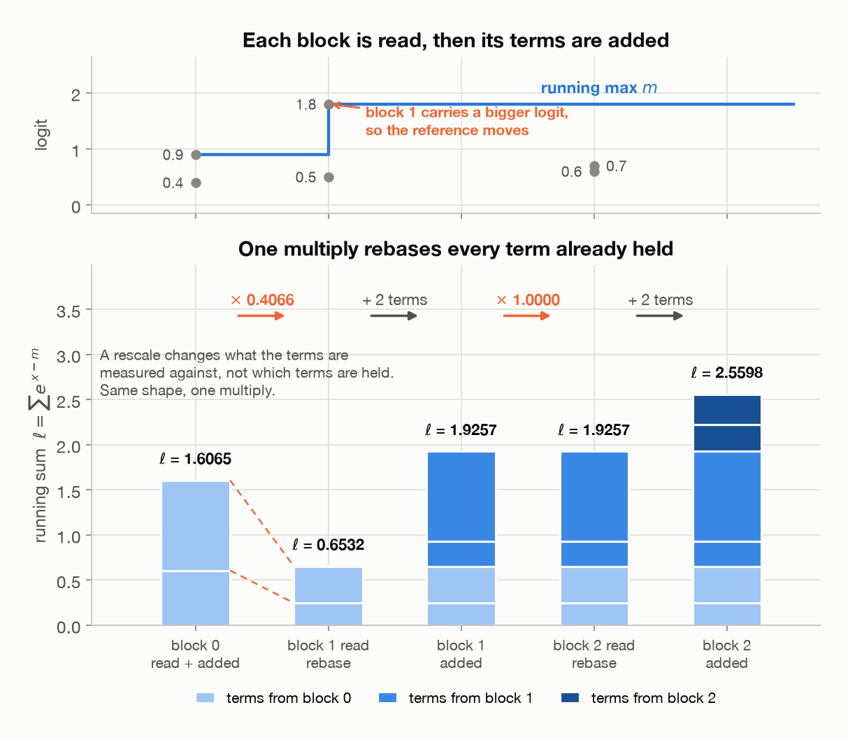
Read it left to right. The loop takes a block, rebases what it is already holding, then adds that block’s own terms. Block 1 contains 1.8, larger than anything seen so far, so the reference $m$ moves from 0.9 up to 1.8 and the two terms already held are multiplied by $e^{0.9 - 1.8} = 0.4066$. The dashed lines carry each term’s boundary across that step, and the stack keeps its proportions exactly, because a single factor hit every piece of it. Block 2’s largest logit is 0.7, which fails to beat 1.8, so its correction is $e^0 = 1$ and its rebase column is a copy of the column before it.
(The loop does the rebase and the add in one statement. They get a column each here because the rebase is the step being argued for.)
Every number in that figure comes from rebase_walkthrough, which streams those six logits through the loop and prints each step’s arithmetic in full. Read l as $\ell$, and exp(a - b) as $e^{a-b}$:
1
2
3
4
5
6
7
8
9
10
11
12
13
14
  block 0   m = 0.9, nothing held yet
    l = exp(0.4 - 0.9) + exp(0.9 - 0.9)
      = 0.6065 + 1.0000
      = 1.6065

  block 1   m: 0.9 -> 1.8, so correction = exp(0.9 - 1.8) = 0.4066
    l = 1.6065 x 0.4066 + exp(0.5 - 1.8) + exp(1.8 - 1.8)
      = 0.6532 + 0.2725 + 1.0000
      = 1.9257

  block 2   m: 1.8 -> 1.8, so correction = exp(1.8 - 1.8) = 1.0000
    l = 1.9257 x 1.0000 + exp(0.6 - 1.8) + exp(0.7 - 1.8)
      = 1.9257 + 0.3012 + 0.3329
      = 2.5598
Three lines, three different situations. Block 0 has no history behind it, so $\ell$ is nothing but its own two terms, each measured against the block’s own max of 0.9. Block 1 is the line the section exists for: 1.6065 x 0.4066 is the entire accumulated history being rebased onto the new reference in one multiplication, and only after that do block 1’s own terms join at that reference. Block 2 carries a max of 0.7, which loses to 1.8, so its correction is $e^0 = 1$ and 1.9257 x 1.0000 leaves the history untouched; the block still contributes its own two terms.
Each line adds up in the digits printed, so any of them can be checked on a calculator, including the multiplication.
Block 1 is also where the derivation above can be checked rather than believed. Rescaling the running total by one factor, against recomputing both held terms from scratch at the new reference:
1
2
3
  one multiply: l_old x correction   0.6532
  recomputed: sum exp(x - m_new)     0.6532
  difference                         0.0000
And after all three blocks, what the streaming version accumulated against what the ordinary version computes with the whole row in hand:
1
2
3
  streamed sum after 3 blocks        2.5598
  one-shot sum exp(x - max)          2.5598
  difference                         0.0000
Nothing in the derivation was specific to the normalizer. Any running quantity built as a sum of terms sharing the reference $m$ can be rebased by the same multiply, which is why the tiled loop in §4 rescales its output accumulator with the identical factor.
In code, the normalizer version is nine lines. This is online_softmax’s first pass, with the device and dtype plumbing removed:
1
2
3
4
5
6
7
8
9
m = torch.full((*lead, 1), float("-inf"))
l = torch.zeros((*lead, 1))

for start in range(0, n, block_size):
    block = x[..., start : start + block_size]
    m_new = torch.maximum(m, block.max(dim=-1, keepdim=True).values)
    correction = torch.exp(m - m_new)
    l = l * correction + torch.exp(block - m_new).sum(dim=-1, keepdim=True)
    m = m_new
Note l * correction. When the max doesn’t change, correction is $e^0 = 1$ and costs nothing. When it does, it fixes the entire accumulated history in one multiply.
How often does it fire?
Cheap is not free, so the remaining question is how often a block raises the max at all. Streaming a real row of 2,048 logits past the same loop, 64 at a time:
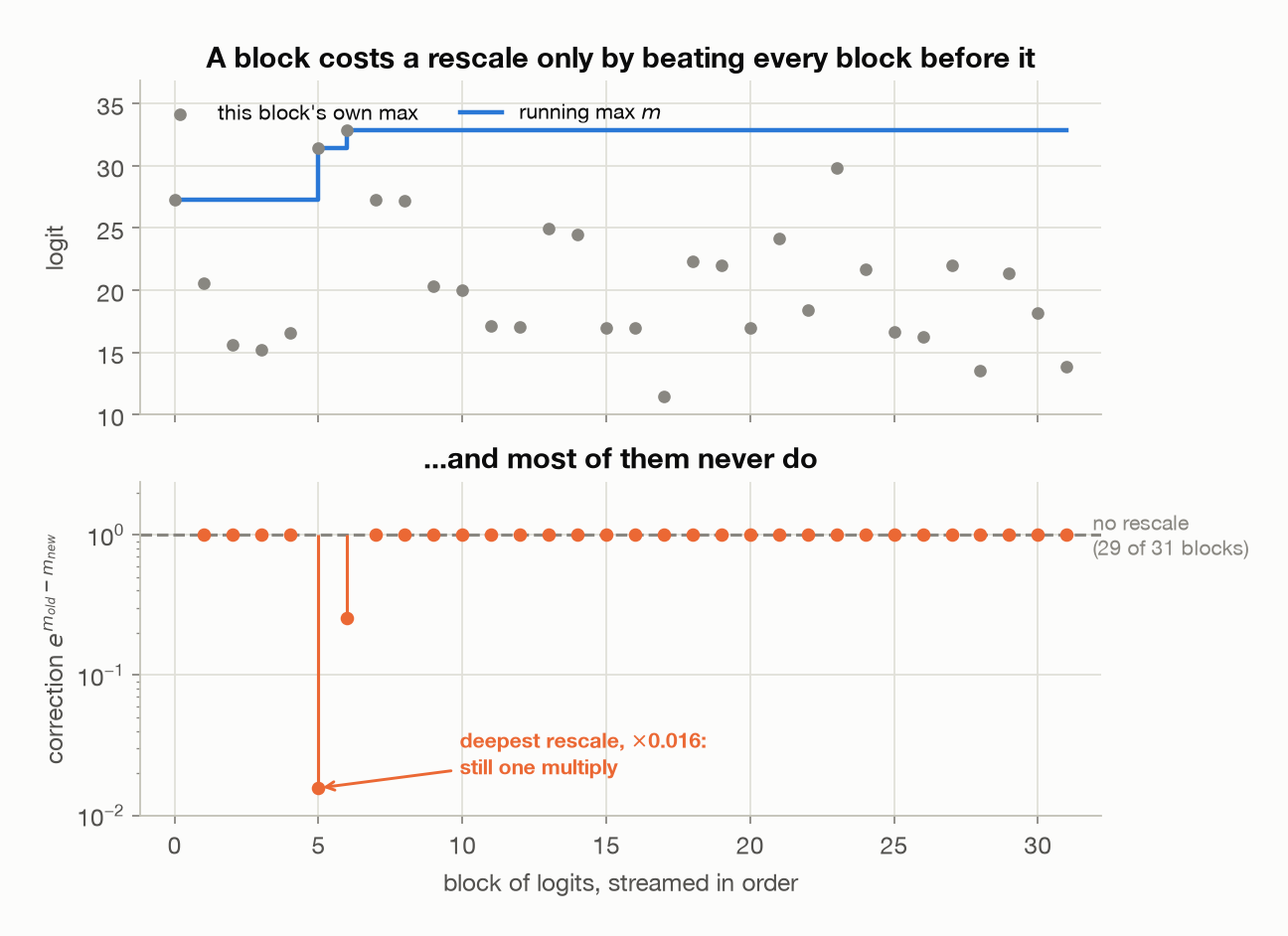
The top panel is the reason the bottom one is nearly empty. A block forces a rescale only by beating every block before it, and a running maximum gets harder to beat the longer it runs, so the two blocks that cost anything on this run both land in the first six, and the other 29 cost exactly nothing. The deepest correction, $\times 0.016$, is still a single multiply applied to one accumulator, not a second pass over the data.
3. Partial softmaxes compose
Does it actually agree with torch.softmax? check_online_softmax draws four rows of 2,048 logits and multiplies them by 8, which stretches each row to span about 58. That is a deliberately hostile input: across a range that wide the largest exponential is $e^{58}$ times the smallest, so any weakness in the rescaling has room to show. It then runs the loop above at four block sizes and compares every output against PyTorch’s own softmax.
The error is reported two ways, in scientific notation and in ulps, and the ulp column is the one to read. An ulp is a unit in the last place: the gap between one number a format can represent and the next one up. It is the smallest difference floating-point arithmetic can even express, so measuring an error in ulps says how many representable steps apart two answers are — and one or two steps means “as close as fp32 can get”. At the scale of the largest probability here, that step is $2^{-24}$.
1
2
3
4
5
6
7
8
9
  logit row range (max - min)        58.0
  largest probability in a row       0.7605

  block size  max |online - torch|  in ulps  rows sum to
  --------------------------------------------------------
  64                     1.788e-07      3.0       1.0000
  128                    8.941e-08      1.5       1.0000
  512                    1.192e-07      2.0       1.0000
  2048                   1.192e-07      2.0       1.0000
The last block size, 2,048, is the whole row at once: one block, no streaming, nothing to rescale. It is the control, and the other three sit beside it.
Every block size lands between one and a half and three of those steps away from PyTorch. Read as raw digits the column looks like it wanders, 64 worse than 128 and then 512 worse again, but there is no trend in it. Summing the same numbers in a different order shuffles the last bit or two, and that is all this column is able to detect.
Those digits are one of only two numbers in this post that will not reproduce exactly on your machine, the other being §8’s wall-clock timings. Each backend sums in its own order, so the same run on CPU lands at 3 to 4 ulps rather than 1.5 to 3. The logits themselves are drawn on CPU and then moved to the device, which is why the row range and the largest probability above are identical everywhere. What varies is the last bit or two of the comparison, and the claim was never about those.
The rows still sum to 1, which is the other half of the check: the rescaling could in principle preserve the ratios between outputs while getting the normalizer wrong, and that column would catch it. Block size changes the memory schedule, not the answer — the property everything else in this post rests on.
And the running max — what is it for?
The usual story — “without it the exponentials overflow” — is not quite true, and it is easy to repeat without checking. Compare against the naive exp(x)/sum(exp(x)) at both precisions — the number formats the arithmetic runs in, fp32 being 32 bits per number and fp16 sixteen:
1
2
3
4
5
6
for label, dtype in (("fp32", torch.float32), ("fp16", torch.float16)):
    xd = x.to(dtype)
    e = torch.exp(xd)                               # the naive way: no max subtracted
    naive = e / e.sum(-1, keepdim=True)
    overflow_at = math.log(torch.finfo(dtype).max)  # past here, exp stops fitting
    bad = int(torch.isinf(e).sum() + torch.isnan(naive).sum())
The exp overflows past column is nothing but log of the largest number each format can hold, so it is a fact about the format and not about these logits: fp32 tops out near $3.4 \times 10^{38}$, fp16 at 65,504.
1
2
3
4
  dtype  exp overflows past  actual row max  overflowed?  bad values  naive error
  ---------------------------------------------------------------------------------
  fp32                 88.7            32.8           no           0    1.192e-07
  fp16                 11.1            32.8          yes       1,320          nan
In fp32, exp overflows only past $x \approx 88.7$, and a row max of 32.8 isn’t close — the unstable version survives these logits perfectly well, matching to about one ulp. In fp16 the threshold drops to $x \approx 11.1$, the same logits overflow 1,320 times, and every one becomes a nan.
So the max subtraction is not guarding against an overflow that fp32 was ever going to hit. It earns its place at the precision inference actually runs in. That matters for Flash Attention specifically: the running max is what lets the algorithm carry the same guarantee per tile, at whatever precision the kernel is compiled for, without ever seeing the whole row.
4. Tiled attention in 40 lines
Now build attention on it. Outer loop over query blocks; inner loop streams key/value blocks past them, updating the running statistics and the accumulated output:
1
2
3
4
5
6
7
8
9
10
11
12
13
14
15
16
17
18
19
20
21
for i in range(0, seq_q, block_q):
    qi = q[:, :, i : i + block_q]
    rows = qi.shape[2]                 # this block's height
    m = torch.full((batch, heads, rows, 1), float("-inf"))
    l = torch.zeros((batch, heads, rows, 1))
    acc = torch.zeros((batch, heads, rows, dim))

    for j in range(0, seq_k, block_k):
        kj, vj = k[:, :, j : j + block_k], v[:, :, j : j + block_k]
        cols = kj.shape[2]             # and this one's width
        scores = (qi @ kj.transpose(-2, -1)) * scale

        m_new = torch.maximum(m, scores.max(dim=-1, keepdim=True).values)
        correction = torch.exp(m - m_new)
        p = torch.exp(scores - m_new)

        l = l * correction + p.sum(dim=-1, keepdim=True)
        acc = acc * correction + p @ vj   # rescale history, then add this tile
        m = m_new

    out[:, :, i : i + block_q] = acc / l
The line that carries the algorithm is acc = acc * correction + p @ vj. The accumulated output — not just the normalizer — has to be rebased when the max moves. Miss that and you get a plausible-looking result that is quietly wrong.
Also notice the division by l happens once at the end, outside the inner loop. You accumulate an unnormalized weighted sum and normalize last, which is what makes the accumulation associative.
5. Exact, and what “exact” is worth
check_exactness runs the tiled implementation against F.scaled_dot_product_attention — PyTorch’s built-in attention, usually shortened to SDPA, which dispatches to the best kernel it has for your hardware — across tile shapes. Both settings of causal masking are checked. That is the look-only-backwards rule from the short version, the thing that stops a language model reading ahead to the answer, and it is implemented by forcing the scores above the diagonal to $-\infty$ so the softmax sends them to zero. §7 shows what tiling does with it.
1
2
3
4
5
6
7
8
9
10
11
12
13
14
15
  causal=False: tiled vs F.scaled_dot_product_attention

  tile (q x k)  max abs difference
  ----------------------------------
  64 x 64                4.768e-07
  128 x 128              5.066e-07
  256 x 512              4.917e-07

  causal=True: tiled vs F.scaled_dot_product_attention

  tile (q x k)  max abs difference
  ----------------------------------
  64 x 64                1.431e-06
  128 x 128              1.431e-06
  256 x 512              1.431e-06
That’s floating-point reassociation noise: adding the same numbers in a different order gives a very slightly different answer, because each intermediate rounding lands differently. Tiling adds them in a different order, so a difference at the last bit or two is expected — the same order as post 1’s check. The tile shape doesn’t move it, because the tile shape isn’t part of the math.
Now the comparison that gives “exact” its meaning. Sliding-window attention is a genuine approximation — each query attends only to the last $w$ keys:
1
2
3
4
5
6
7
def sliding_window_attention(q, k, v, window: int):
    scale = 1.0 / math.sqrt(q.shape[-1])
    scores = (q @ k.transpose(-2, -1)) * scale
    pos = torch.arange(scores.shape[-1], device=q.device)
    too_old = (pos[None, :] < pos[:, None] - window + 1) | (pos[None, :] > pos[:, None])
    scores = scores.masked_fill(too_old, float("-inf"))
    return torch.softmax(scores, dim=-1) @ v
That too_old mask is the only difference. It throws away scores the exact version keeps, so what comes out the other end is a different function — and the table below is measuring how different:
1
2
3
4
5
  method                 max abs difference vs exact
  ----------------------------------------------------
  Flash / tiled (exact)                    1.431e-06
  sliding window, w=256                       0.6047
  sliding window, w=64                        1.5660
Five orders of magnitude, and the distinction behind them is the one to hold onto. Sparse attention, linear attention and low-rank attention all change the function being computed, so with any of them you have to evaluate whether the change costs you anything. Flash Attention changes only the order of memory accesses, so there is nothing to evaluate; if it produced different results, it would be a bug.
6. The memory that never gets allocated
memory_scaling does the measuring, and it takes a little care, because an allocator reuses memory the instant nothing points at it any more — run naive attention and drop the result, and the $n \times n$ matrix can vanish from the peak reading before you ever see it. So the naive path’s score matrix is deliberately held alive across the measurement:
1
2
3
4
5
6
reset_peak_memory(device)
base = peak_memory_bytes(device) or 0
_, weights = naive_attention(q, k, v, causal=True)   # keep the n x n matrix referenced
sync(device)
naive_bytes = (peak_memory_bytes(device) or 0) - base
del weights
The tiled path is measured by the same four lines with flash_attention in the middle and nothing held. Two of the four columns below come out of that; the other two are arithmetic, not measurement. Score matrix is $H \cdot n^2 \cdot 4$ bytes — 8 heads, four bytes per fp32 number — and one tile is the same expression with $n^2$ replaced by the tile’s $128 \times 128$:
1
2
3
4
5
6
7
8
9
  seq   score matrix (n^2)  naive measured  one tile  tiled residual
  --------------------------------------------------------------------
  512              8.0 MiB         9.0 MiB   0.5 MiB         0.0 MiB
  1024            32.0 MiB        33.0 MiB   0.5 MiB         0.0 MiB
  2048           128.0 MiB       130.0 MiB   0.5 MiB         0.0 MiB
  4096           512.0 MiB       524.0 MiB   0.5 MiB         0.0 MiB

  8x the sequence, score matrix grows 64x
  tile size, independent of sequence 0.5 MiB
So columns two and four are analytic, columns three and five are measured, and the point of putting them side by side is that they agree. The measured naive column tracks the analytic $n^2$ column to within a couple of MiB, which is the check that the formula describes what the machine actually does. The tiled residual is 0 because each tile is freed as the loop advances — that’s the claim, not a measurement artifact; the meaningful number is the constant 0.5 MiB in column four.
And that constant is where §1’s 192 KB comes back. The 0.5 MiB is a $128 \times 128$ tile across all 8 heads at once; per head it’s 64 KiB, and a head is what one streaming multiprocessor works on. So the tile was sized to fit an SM’s private scratchpad with room to spare — that’s the constraint the block size is chosen against, and why it’s a constant rather than a function of $n$.
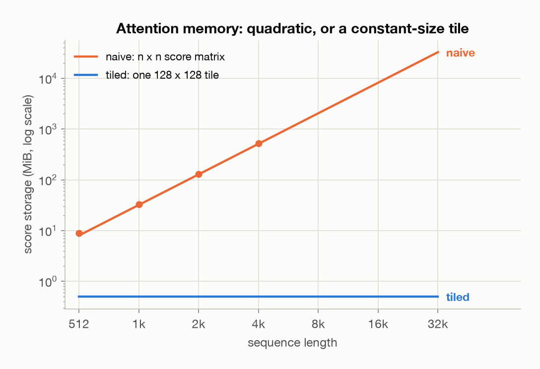
Extrapolating past what my laptop can hold — the same $H \cdot n^2 \cdot b$ bytes, now with nothing measured, because none of these would fit. The second column swaps the demo’s shape for a real one: Llama 3.1 8B has 32 query heads against the demo’s 8 and runs in bf16 rather than fp32, which is four times the heads against half the bytes, so twice the matrix.
1
2
3
4
5
6
7
8
9
10
  seq     8 heads, fp32  Llama 3.1 8B: 32 heads, bf16
  -----------------------------------------------------
  8192          2.0 GiB                       4.0 GiB
  16384         8.0 GiB                      16.0 GiB
  32768        32.0 GiB                      64.0 GiB
  131072      512.0 GiB                    1024.0 GiB

  At 128k in Llama 3.1 8B's shape that is 1.0 TiB of scratch for a
  single layer - enough to fill about 14 A100 80GB cards, holding a
  matrix that is normalized and thrown away immediately.
A terabyte, for one layer, for a matrix that exists only long enough to be normalized. And post 2 measured that same model needing 16 GiB of KV cache per user at the same context length — so before Flash Attention, attention wanted sixty-four times a user’s entire cache as transient scratch, on top of the cache itself.
This is why long context was infeasible before 2022 — not because the FLOPs were unaffordable, but because you could not allocate the intermediate. Getting memory from $O(n^2)$ down to $O(n)$ is what unlocked it, and Rabe & Staats, Self-attention Does Not Need $O(n^2)$ Memory (2021), had made the same point a year earlier from the memory side alone, without the IO-aware kernel that turned it into a speedup — IO-aware meaning written around the cost of moving data rather than the cost of arithmetic, which is the design stance this post has been describing.
This is not the KV cache
A warning, because the two big memory numbers in this series are easy to confuse. Post 2 measured a KV cache of 16 GiB per user at 128k context. This post measures a score matrix of 512 GiB at 128k. Same context length, wildly different numbers, and they are different memory doing different jobs:
| KV cache (post 2) | Score matrix (this post) | |
|---|---|---|
| What it holds | keys and values for every token so far | every query scored against every key |
| Lives for | the whole conversation | one layer, one forward pass |
| Grows with | tokens, linearly | tokens, quadratically |
| Per user? | yes, one cache each | no, transient scratch |
| Fixed by | GQA, quantization, paging | Flash Attention |
Flash Attention removes the second and does nothing whatsoever to the first. If you are sizing a deployment, the cache is still the line item that decides how many users fit on a card — that was post 2’s §8. What this post buys you is that attention no longer needs a quadratic scratch buffer on top of the cache, which is what made 128k context feasible to run at all.
7. Causal masking gets a bonus
causal_skipping counts what that buys. Once you’re looping over tiles, causal masking stops being a masked_fill and becomes a scheduling decision. If a key block starts after the query block ends, every score in that tile would be $-\infty$. So don’t compute it:
1
2
3
if causal and j > i + rows - 1:
    counters["blocks_skipped"] += 1
    continue
1
2
3
4
5
  block size  tiles computed  tiles skipped  fraction skipped
  -------------------------------------------------------------
  128                    136            120               47%
  256                     36             28               44%
  512                     10              6               38%
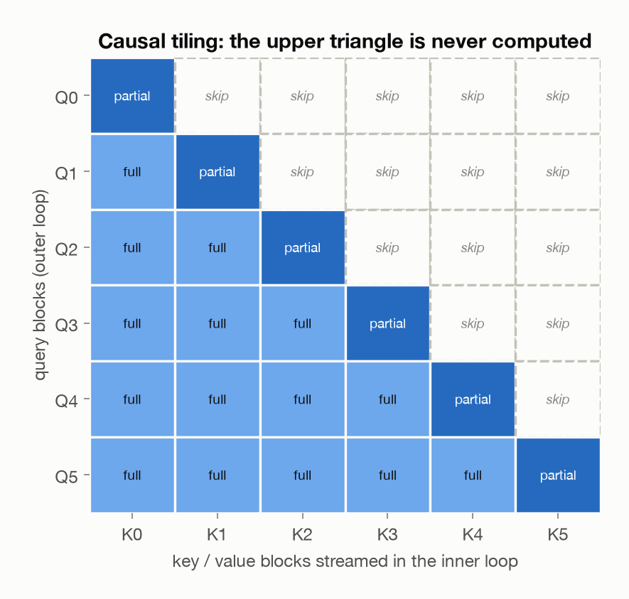
Just under half the work disappears. The naive path computes that entire upper triangle, writes it to HBM, reads it back, and softmaxes it into zeros. Only the diagonal tiles need an actual mask — everything below is fully visible, everything above is skipped outright.
Nothing in that table is a measurement. It is a tile count, so it comes out identical on any machine, and it has a closed form: with $B = n/\text{block}$ blocks along each side, the loop computes the lower triangle including the diagonal, $B(B+1)/2$ tiles out of $B^2$, and skips
\[\frac{B^2 - B(B+1)/2}{B^2} = \frac{B-1}{2B}\]At 2,048 tokens that is $15/32 = 46.9\%$ for block=128, $7/16 = 43.8\%$ for 256, and $3/8 = 37.5\%$ for 512 — the three rows above. That is also why smaller blocks skip more: the diagonal they are forced to compute is a thinner slice of the matrix, one row of tiles in sixteen at block=128 against one in four at block=512. The ceiling is 50%, approached and never reached, because the diagonal always has to be computed.
8. Where the speed actually comes from
First: it is not from doing less arithmetic
This post has been asserting that the win is memory traffic rather than FLOPs. That’s a comparison, so it needs both quantities in one table, which is what flops_vs_bytes assembles.
The tiled column is tallied as the loop runs rather than derived afterwards — one line inside the inner loop, incremented on every tile actually computed, so tiles the causal skip drops never get counted:
1
counters["matmul_flops"] += 2 * (2 * batch * heads * rows * cols * dim)
Two matmuls (matrix multiplies) per tile, $QK^\top$ and $PV$; each costs $2 \cdot \text{rows} \cdot \text{cols} \cdot d$, the factor of two being one multiply and one add per element accumulated. The naive column is that same expression with the tile replaced by the whole matrix, and the traffic column counts the score matrix crossing HBM on the passes §1 listed — write $S$, read $S$, write $P$, read $P$, four crossings of $H \cdot n^2 \cdot 4$ bytes. At $n = 4096$:
\[\underbrace{2 \times (2 \cdot 8 \cdot 4096^2 \cdot 64)}_{34.4\ \text{GFLOP}}, \qquad \underbrace{4 \times 8 \times 4096^2 \times 4\ \text{B}}_{2048\ \text{MiB}}\]Both columns are counted, not timed; they reproduce exactly on any machine. With causal masking off, where both paths must touch every position:
1
2
3
4
5
6
  seq   naive FLOPs  tiled FLOPs  ratio  naive score traffic  tiled
  -------------------------------------------------------------------
  512         0.5 G        0.5 G  1.00x               32 MiB  0 MiB
  1024        2.1 G        2.1 G  1.00x              128 MiB  0 MiB
  2048        8.6 G        8.6 G  1.00x              512 MiB  0 MiB
  4096       34.4 G       34.4 G  1.00x             2048 MiB  0 MiB
The FLOP columns are equal to the digit — the tiled path does not save a single multiply. What it removes is the third column: 2 GiB of score traffic at 4k context, gone, because the tile never leaves the accumulator.
That is the trade, and it explains the shape of everything else here: FLOPs and score traffic both grow as $n^2$, and after tiling only one of them is still being paid.
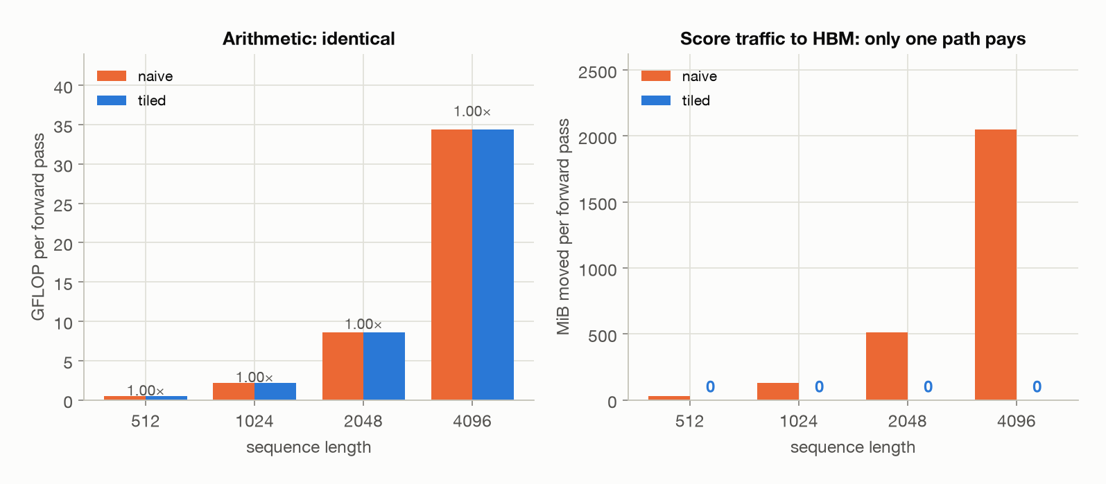
Two panels, because the two quantities have nothing to do with each other dimensionally and the contrast between them is the result: same bars on the left, one bar missing entirely on the right.
The traffic that doesn’t go away
That 0 MiB column is score traffic, and reading it as all traffic overstates the case. The tiled path still reads $Q$, $K$ and $V$ in from HBM and writes $O$ back out — and because the inner loop streams the whole of $K$ and $V$ past every query block, $K$ and $V$ get re-read once per query block. Count every tensor that crosses HBM rather than only the score matrix:
1
2
3
4
5
6
  seq   naive: all tensors  tiled: all tensors  reduction  K/V re-reads
  -----------------------------------------------------------------------
  512               36 MiB              10 MiB       3.6x            4x
  1024             136 MiB              36 MiB       3.8x            8x
  2048             528 MiB             136 MiB       3.9x           16x
  4096            2080 MiB             528 MiB       3.9x           32x
Counted the same way as the FLOPs, one line inside the loop, so skipped tiles cost nothing:
1
counters["hbm_bytes"] += 2 * batch * heads * cols * dim * elem
If it helps to have a picture for the whole thing: a cook making a thousand sandwiches, with the fridge down the hall. The slow version fetches bread, walks back, puts it away, fetches cheese, walks back. The cook is quick; almost all the elapsed time is corridor. The fix is to carry a tray of ingredients to the counter and finish several sandwiches before going back. The cooking takes just as long either way, and what shrinks is the walking. Flash Attention is the tray.
So the honest figure is about 4×, not infinity. What Flash Attention removes is the quadratic intermediate; what it pays back is re-reading $K$ and $V$ once per query block, which is why the reduction settles near 4× instead of growing without bound. That is also why block size is a real tuning knob rather than an implementation detail: a bigger query block means fewer re-reads of $K$ and $V$, and a bigger tile to keep resident in a scratchpad that has 192 KB to spare.
The two columns answer different questions, and both matter. The score column is why the memory goes from $O(n^2)$ to $O(n)$ — §6’s result, and the reason long context became possible at all. This column is why the time improves by the factor the timing table below shows rather than by a factor of a thousand.
Turn causal masking on and the tiled path does strictly less of both, because of the skipped blocks from §7:
1
2
3
4
5
6
  seq   naive FLOPs  tiled FLOPs  ratio  naive score traffic  tiled
  -------------------------------------------------------------------
  512         0.5 G        0.3 G  0.62x               32 MiB  0 MiB
  1024        2.1 G        1.2 G  0.56x              128 MiB  0 MiB
  2048        8.6 G        4.6 G  0.53x              512 MiB  0 MiB
  4096       34.4 G       17.7 G  0.52x             2048 MiB  0 MiB
That ratio column isn’t measured either — it’s §7’s tile count seen from the other side, $\frac{B+1}{2B}$ of the naive arithmetic. The 0.53 row is exactly §7’s 47%, both at 2,048 tokens with block=128; by 4,096 tokens $B$ has doubled and it has tightened to 0.52, still creeping toward one half.
These are two different kinds of saving. The arithmetic saving is a bonus that tiling makes available; removing the traffic is the mechanism, and Flash Attention would still be worth using at ratio 1.00.
Then: why the loop above is still slow
An honest caveat: the Python tiled loop is slower than naive attention. Every tile still round-trips through HBM, plus Python overhead per iteration. The algorithm is what buys the memory, and fusing it into a single kernel is what buys the time.
So for timing, compare naive attention against F.scaled_dot_product_attention, which dispatches to exactly the fused kernel §1 described. Two warmup passes, then the median of five — the first call on this machine pays for shader compilation (on an NVIDIA box it would be CUDA context creation), either of which can run 100× the steady-state cost and would swamp a plain average:
1
2
3
4
naive_ms = benchmark_ms(lambda: naive_attention(q, k, v, causal=True),
                        device=device, warmup=2, repeats=5)
fused_ms = benchmark_ms(lambda: F.scaled_dot_product_attention(q, k, v, is_causal=True),
                        device=device, warmup=2, repeats=5)
timing produces this one, and it is wall-clock on my laptop. Along with §3’s error column it is one of only two tables here that will not reproduce digit for digit on your machine, and it is by far the looser of the two, so read the shape rather than the digits:
1
2
3
4
5
6
  seq   naive (ms)  fused SDPA (ms)  speedup
  --------------------------------------------
  512       1.2076           0.3503    3.45x
  1024      3.6293           0.8023    4.52x
  2048     13.0302           2.0358    6.40x
  4096     56.8895           6.9739    8.16x
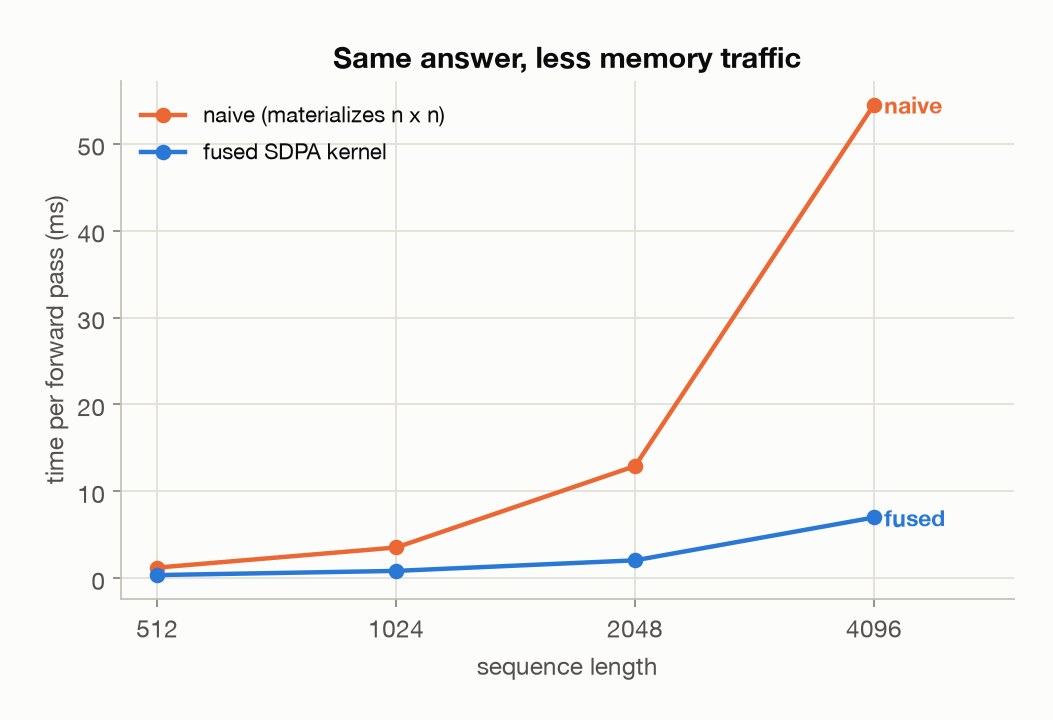
The speedup grows with sequence length, from about 3.5× at 512 tokens to about 8× at 4,096, because the naive path’s memory traffic grows quadratically while the fused path’s grows linearly. There is no reason for that to stop at 4,096. (Wall-clock again, so the exact multiples move a little between runs; the widening is the part that holds.)
One more piece: the backward pass. Training normally stores the attention probabilities for the backward pass, which is the $O(n^2)$ tensor you just avoided allocating. Flash Attention instead recomputes the tiles during the backward pass from $Q$, $K$, $V$ and the saved statistics. Recomputation sounds expensive until you notice which resource it spends: arithmetic, the one in surplus. Redoing the FLOPs costs less than storing the result and reading it back.
A note on versions, since interviews tend to ask for the specifics. Two more pieces of vocabulary make it readable: a warp is the group of 32 GPU threads that execute in lockstep, the unit work gets divided into; tensor cores are the dedicated circuits that do matrix multiplies, separate from the general-purpose arithmetic units beside them.
FlashAttention-2 (2023) improved how work is partitioned across warps and cut the number of non-matmul FLOPs. That sounds like a strange thing to optimize until you see the gap it exploits: on an A100 the tensor cores do 312 TFLOP/s of FP16 matmul against 19.5 TFLOP/s of non-matmul FP32 (a TFLOP/s being a trillion floating-point operations a second), so as the paper puts it, “each non-matmul FLOP is 16× more expensive than a matmul FLOP.” Rescalings and sums are exactly the non-matmul work online softmax adds, which is why trimming them mattered.
FlashAttention-3 (2024) targets Hopper hardware: asynchronous memory copies through the TMA (Tensor Memory Accelerator, a unit that moves tiles between HBM and SRAM without occupying the compute threads), warp specialization so different warps handle copying and computing, and FP8.
Everything this post measured, in one table
All at $n = 4096$, 8 heads, fp32, from the run above:
| Naive | Tiled / fused | Change | |
|---|---|---|---|
| Function computed | attention | the same attention | agree to 1.4e-6 |
| FLOPs, causal off | 34.4 G | 34.4 G | 1.00× — none saved |
| FLOPs, causal on | 34.4 G | 17.7 G | 0.52×, a bonus from tiling |
| Peak score memory | 512 MiB | 0.5 MiB | $O(n^2) \to$ constant |
| Score traffic to HBM | 2048 MiB | 0 MiB | eliminated |
| Total HBM traffic | 2080 MiB | 528 MiB | 3.9× |
| Wall clock | 56.9 ms | 7.0 ms | 8.2× |
Read down the rows and the pattern is plain enough: the function is unchanged, the FLOPs are unchanged, and everything about memory moves. Flash Attention does not compute less, it moves less — and on hardware where attention spends its time waiting on memory, moving less is what being faster amounts to.
9. Sidebar: the probe
One question to close on — the kind this material gets asked, and what separates an answer that sounds right from one that is.
“Does Flash Attention change your model’s output?”
A weak answer: “It’s an approximation that trades a little accuracy for a big speedup on long sequences.”
This is wrong, and it’s a common wrong answer — the name sounds like the efficient-attention family (Linformer, Performer, Longformer), which are approximations.
A stronger answer: “No. It’s exact — an IO-aware reordering of the same computation. It tiles Q, K and V so the score tiles stay in SRAM, and uses online softmax with a running max and sum so partial results compose. Outputs match a naive implementation to floating-point reassociation noise, around 1e-6 in fp32; I’ve measured it. It doesn’t even do less arithmetic — non-causal, the FLOP counts are identical to the digit. What it removes is the quadratic score traffic to HBM, which is why memory goes from $O(n^2)$ to $O(n)$ and why long context became feasible. That’s the opposite of sparse or linear attention, which genuinely change the function — sliding-window attention differs from exact attention by about 0.6 on the same test, five orders of magnitude more than Flash does.”
The tell is whether someone distinguishes it from the approximate-attention family, and whether they know the mechanism is online softmax rather than “it’s optimized CUDA.”
What’s next
Next in the series — planned as post 4 — is quantization, where the tradeoff is real: fewer bytes per weight genuinely does lose information, and the interesting question is what breaks first. The plan is to implement INT8 and NF4 by hand, watch per-tensor scaling get destroyed by a single outlier channel, and work out why perplexity is a misleading way to decide whether a quantized model is safe to ship.
Appendix: all notation
Every symbol this post uses, in one place. Post 1’s appendix covers the ones inherited from attention itself in more depth, and post 2’s the ones about serving.
| Symbol | Means | In this post’s runs |
|---|---|---|
| $n$ | tokens in the sequence — the quantity everything here scales in | 512–4,096 measured, 128k extrapolated |
| $d$ | numbers in one query, key or value vector (the head dimension) | 64 |
| $H$ | attention heads computed side by side | 8 |
| $Q$, $K$, $V$ | the query, key and value matrices, one row per token | $n \times d$ each |
| $S = QK^\top$ | every query scored against every key — the score matrix | $n \times n$ |
| $P = \text{softmax}(S)$ | those scores turned into weights that sum to 1 along each row | $n \times n$ |
| $O = PV$ | the output: each token’s values averaged by its weights | $n \times d$ |
| $x_i$, $x_j$ | single entries of one row on its way through a softmax | — |
| $m$ | the running max, carried across blocks; $m_{\text{old}}$ and $m_{\text{new}}$ are it before and after a block | one number per query row |
| $\ell$ | the running sum — the softmax denominator — rebased whenever $m$ moves | one number per query row |
| $e^{m_{\text{old}} - m_{\text{new}}}$ | the correction factor that rebases everything already accumulated | exactly 1 for 29 of 31 blocks |
block, block_q, block_k | the tile’s edges: how many queries and how many keys one tile covers | $128 \times 128$ unless stated |
| rows, cols | the tile actually in hand, which is smaller at the end of a sequence | $\le 128$ |
| $B$ | blocks along one side of the score matrix, $B = n/\text{block}$ | 4–32 |
| $w$ | window width in sliding-window attention — the approximation used for contrast | 64, 256 |
| $O(n^2)$, $O(n)$ | how memory grows with sequence length: with its square, or in step with it | — |
| FLOP, GFLOP | one floating-point add or multiply; $10^9$ of them | 0.5–34.4 G per pass |
| fp32, fp16 | 32- and 16-bit floating point — four and two bytes a number | fp32 unless stated |
| KiB, MiB, GiB | 1024, $1024^2$, $1024^3$ bytes — what an allocator reports | every computed figure |
Three things worth keeping straight, because the post leans on all of them:
- $O$ is overloaded, and unavoidably so. $O = PV$ is attention’s output matrix; $O(n^2)$ is growth notation. They are unrelated, both are standard, and both appear here. Context separates them — an $O$ on its own is the output, an $O$ with a parenthesised expression is a rate.
- KB and MB against KiB and MiB. The A100 figures in §1 (192 KB per SM, ~20 MB total, 40–80 GB of HBM) are quoted exactly as the vendor publishes them. Every number this post computes or measures is binary: KiB, MiB, GiB, powers of 1024, because that is what an allocator reports. §6 puts a 64 KiB tile next to a 192 KB scratchpad; that comparison survives either reading of “KB”, since the tile fits with about threefold room to spare on both.
- $n$ here is one length, not two. Post 2 split a sequence into prompt $p$ and generated tokens $n$, because generation makes that split matter. This post is about a single forward pass over $n$ tokens, queries and keys the same length, which is why the score matrix is square.
References
- Dao et al., FlashAttention: Fast and Memory-Efficient Exact Attention with IO-Awareness (2022) — the paper this post reimplements. “Exact” is in its title.
- Dao, FlashAttention-2: Faster Attention with Better Parallelism and Work Partitioning (2023) — §8’s version notes. The 16× figure is its §3.1: 312 TFLOP/s of matmul against 19.5 TFLOP/s of non-matmul on an A100.
- Shah et al., FlashAttention-3: Fast and Accurate Attention with Asynchrony and Low-precision (2024) — the Hopper-specific work in §8.
- Milakov & Gimelshein, Online normalizer calculation for softmax (2018) — where §2’s running-statistics trick comes from, four years before Flash Attention put it to this use.
- Rabe & Staats, Self-attention Does Not Need $O(n^2)$ Memory (2021) — §6’s point, made a year earlier without the fused kernel.
- Code for this post:
llm-architectures-refresher,uv run demo03.