LLM Architecture Refresh [2]: The KV Cache, and Why Decode Is Memory-Bound
Measuring the KV cache — why generation is quadratic without it, why the cache outgrows the model weights at long context, and why decode is memory-bandwidth-bound while prefill is compute-bound.
The number that decides what you can serve
Post 1 was about how attention works. This one is about the single fact that determines what you can actually deploy: generating a token is a fundamentally different workload from reading one, and almost every inference optimization you’ve heard of follows from that one asymmetry.
The short version
First, what the thing actually is, because the name is worse than the idea. A model writes text one token at a time — roughly a word — and to pick each new token it looks back over everything written so far. For every earlier token it needs two lists of numbers that it worked out when it first read that token: the token’s key and its value. The token being written makes a third list of its own, its query, which is what it does the looking with. (Post 1 covers where all three come from and what they mean. Here, all that matters is that keys and values exist, and that once computed they never change.)
Keeping those keys and values around instead of recomputing them at every step is the KV cache. That’s it — not a model, not an algorithm, not a clever approximation. A box of numbers you hold onto so you don’t have to work them out twice.
It turns out that box decides almost everything about what an LLM costs to run. If you read nothing else, these are the things this post establishes — each one measured rather than asserted:
- A cache exists because every generation step re-asks for what the last one built. Producing the next token needs a key and a value for every token so far, so each step wants everything the previous one wanted, plus one more. With nowhere to keep them, wanting them again means building them again: three steps build twelve key vectors where only five are distinct. A query is the opposite — made, used once, never wanted again — which is why it’s a KV cache, not a QKV cache.
- It changes nothing about what the model writes. Generating with the cache and without it produce identical text, word for word — not merely similar. The cache hands back numbers it already worked out; it never estimates them. So if your cached and uncached output ever differ, that is a bug, not a tradeoff.
- Without it, the cost explodes as the text gets longer. Every step would redo the work of every step before it, so the total grows with the square of the length. Writing 512 words after a 64-word prompt means processing 576 tokens with a cache and 163,584 without — a 284× multiplier, all of it work already done once.
- It is a bargain, not free money. You hold at most 2× the memory, and hold it for the whole conversation, to save 200–2000× the compute. What makes the trade worth taking is that the two sides grow at different rates as a conversation gets longer: the memory you spend rises in step with the length, while the work you save rises with its square. The longer the conversation, the better the deal.
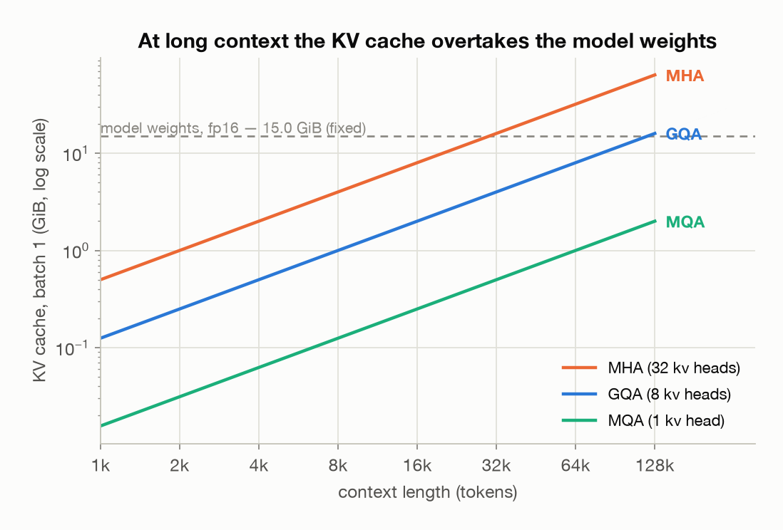
- At long context the cache outgrows the model. A single long conversation on Llama-3-8B needs 16 GiB of cache — against 15 GiB for the model’s own learned parameters, its weights. One copy of the weights serves everybody, but every conversation brings its own cache — so thirty-two concurrent users at that length need half a terabyte, about six 80 GiB GPUs, for a model that fits comfortably on one. “How many users can I serve?” is a KV-cache question, not a model-size question.
- You can store far less without computing any less. Attention runs in parallel lanes called heads, and several lanes can share one set of keys and values rather than each keeping its own. Going from 12 sets down to 1 shrinks the cache 12× while the time per word stays inside a 1.3× band — which is the entire case for grouped-query attention, now the default in new models.
- Generating a token costs about two orders of magnitude more than reading one — 83× per token here. Reading a prompt and writing a reply both haul the model’s entire weights through the chip, but reading spreads that one haul across every token of the prompt at once, while writing pays for it in full, one token at a time. Writing ends up 306× short of the work-per-byte a chip needs to keep its arithmetic busy, so it spends nearly all its time waiting on memory. No amount of clever code closes a gap that size.
- That asymmetry shows up on your bill. Every LLM API charges more for the tokens it writes than for the ones it reads. With Claude it is a flat 5× at every tier, from the cheapest model to the most capable — the input you are billed for is text being read, the output is text being written one token at a time.
- Serving many users at once is nearly free, until abruptly it isn’t. With short prompts, 32 conversations at once cost only 2× the time of one — 16× the output — because they all share a single haul of the weights. Give each of them a 512-token prompt and the same 32 cost 7.5× the time for just 4.3× the output. The weights are shared, but every conversation drags its own cache along, and past a crossover point that unshared half is most of the work.
Every one of those has a receipt behind it — a small program that prints the number, so you can check it rather than take my word. The code lives in a companion repo, llm-architectures-refresher, and runs unchanged on Apple Silicon or a Linux + NVIDIA box:
1
2
3
git clone https://github.com/bearbearyu1223/llm-architectures-refresher
cd llm-architectures-refresher
uv sync && uv run demo02
Every number and figure below came out of that command on my M-series Mac. The Python shown alongside each result is the part that matters, trimmed of setup — the runnable version is in demos/d02_kv_cache.py.
This post needs a real model rather than loose tensors, so the repo gained one: toy_model.py, a Llama-shaped decoder — pre-norm, RMSNorm, RoPE, SwiGLU, no biases, configurable grouped-query attention. It’s small (8–60M parameters) but not wrong, and the later posts on quantization and MoE will reuse it. The weights are random, because everything here measures time and memory, never output quality.
Table of Contents
Skip to the short version for the findings without the derivations.
- Why a cache exists at all
- The cache changes nothing about the output
- Without a cache, generation is quadratic
- How big does the cache actually get?
- Shrinking the cache: GQA, MQA, and what you give up
- Prefill vs decode: the whole ballgame
- The batch sweep, and where it stops working
- A worked example: 1,000 users at 128k
- What follows from all this
- Sidebar: the probe
Plus an appendix of all notation at the end, if a symbol ever goes by without introduction.
1. Why a cache exists at all
Start from what post 1 established, because the cache falls straight out of it.
To compute attention for one token, you need three things: that token’s query, and the key and value of every token it is allowed to look at. Causal masking means “allowed to look at” is “itself and everything before it”. So for token 5:
\[\text{output}_5 \;=\; \sum_{j \le 5} w_{5j} \cdot V_j \qquad \text{where} \qquad w_{5j} \;\propto\; Q_5 \cdot K_j\]Now generate text. Each step appends one token and asks for the next, so the model runs again with a sequence one token longer:
1
2
3
4
5
  step       sequence so far  needs     and     and  predicts
  -------------------------------------------------------------
  1            [The cat sat]     Q3  K1..K3  V1..V3      "on"
  2         [The cat sat on]     Q4  K1..K4  V1..V4     "the"
  3     [The cat sat on the]     Q5  K1..K5  V1..V5     "mat"
Read down the K and V columns. Step 2 needs $K_1, K_2, K_3$ — the same $K_1, K_2, K_3$ step 1 already computed. Step 3 needs them again. Every step recomputes almost everything the previous step just finished computing.
Counting what that table asks for makes the case, and three steps is enough to see it. Add up the K column: step 1 wants three keys, step 2 wants four, step 3 wants five — $3 + 4 + 5 = 12$. But only five distinct keys ever appear in the whole table, $K_1$ through $K_5$. So most of those twelve are the same vector being asked for again:
1
2
3
4
5
  tensor  needed over 3 steps  distinct vectors  repeat reads
  -------------------------------------------------------------
  Q                         3                 3             0
  K                        12                 5             7
  V                        12                 5             7
Look at the last column, and at how differently the two rows behave.
For Q it is zero. Three steps, three queries, and no query is ever wanted twice: $3 - 3 = 0$. A cache would sit there with nothing to hand back.
For K and V it is seven: $12 - 5 = 7$. Seven of the twelve demands are for a vector that some earlier step already produced.
That seven is where counting turns into cost. If you have nowhere to put a vector, asking for it again means building it again — the two are the same act. So without a cache, those seven repeats are seven key vectors computed a second time, from tokens that haven’t changed since the first. With a cache, they’re seven array lookups.
Said as shapes: the Q column is a diagonal, the K column a triangle. The figure below draws exactly that, and the quadratic in §3 is what the triangle costs once the sequence is long rather than three steps.
Why they’re safe to reuse
That only works if those keys and values are genuinely unchanged, and two facts from post 1 guarantee it:
- $K_j$ and $V_j$ depend only on token $j$, its position, and the weights. They’re $W_k$ and $W_v$ applied to one token’s vector, with RoPE applied for position $j$. Appending a token later changes none of the three — the token is what it was, position $j$ is still position $j$, and the weights are frozen because this is inference. (That last clause is doing quiet work. The next subsection is what happens when it stops being true.)
- Causal masking means no token’s representation can depend on anything after it. Token 3 could not see token 4 even in principle, so token 4’s arrival cannot disturb it.
That’s an argument, so let’s check it. Run the model on a 4-token prefix, then on those same tokens plus two more, and compare what each run stored for the first four positions:
1
2
3
4
5
short = KVCache(cfg, 1, device, dtype)
model(tokens[:, :4], start=0, cache=short)   # the first four tokens

long = KVCache(cfg, 1, device, dtype)
model(tokens[:, :6], start=0, cache=long)    # the same four, plus two more
A cache holds one tensor per layer, so cache.k has five axes. Slicing the fourth to :4 keeps every layer, sequence, head and feature, and takes only the token positions the two runs have in common:
1
2
3
4
5
6
                         shape                                       meaning
  ----------------------------------------------------------------------------
  cache.k    (2, 1, 4, 64, 32)  layers, batch, kv_heads, positions, head_dim
  the slice   (2, 1, 4, 4, 32)          same, but only the first 4 positions

  numbers being compared             1,024
Now compare them. Subtract one from the other, take absolute values, and keep the largest — if nothing moved, that largest value is zero:
1
(short.k[:, :, :, :4] - long.k[:, :, :, :4]).abs().max()
1
2
  max |K_short - K_long|             0.0000
  max |V_short - V_long|             0.0000
0.0000 is a rounded display though, so it’s worth the stronger check — exact equality, which rules out a tiny non-zero difference hiding behind the rounding:
1
  torch.equal(K_short, K_long)       yes
Not merely close — identical, across all 1,024 numbers. So recomputing them is pure waste, and storing them is safe.
This is an inference-only structure
If you’ve come at this from the training side, the first thing to wonder is whether any of it applies there. It doesn’t: there is no KV cache during training. Two reasons, and either one alone would settle it.
There would be nothing to reuse. Teacher forcing hands the model the entire real sequence before the pass begins, so a training step is one forward pass that computes $K_1 \ldots K_n$ once and lets the causal mask do the rest. Run this section’s count against a training step and there is nothing left to save:
1
2
3
4
                       K vectors computed  of them, redundant
  -------------------------------------------------------------
  generation, 3 steps                  12                   7
  training, 1 pass                      5                   0
Over the same five token positions, an uncached generation run computes twelve key vectors, seven of which redo work it has already done. A training pass computes five and redoes nothing.
Neatly, both rows come straight out of the table above. The generation row is its “needed” and “repeat reads” columns; the training row is its “distinct vectors” column written down twice, because computing each vector exactly once is all a single pass ever does. Training already sits at the floor that caching is trying to reach.
Which gets at what a cache is actually for. It saves work that would otherwise be repeated from one call to the next, and training makes exactly one call. You’d fill it and never read it.
(One thing here looks like reuse and isn’t. Inside that single pass, $K_j$ is attended to by every query position from $j$ onward, so it gets consulted many times over. But consulting is not computing. Those consultations are all one $QK^\top$ matmul, which reads each $K_j$ out of memory a single time. Sharing a value inside one matmul is free; rebuilding it on a later call is what costs, and rebuilding is the only thing a cache prevents.)
And the premise above would be false anyway. Fact 1 said $K_j$ and $V_j$ depend on the token, its position, and the weights. Training changes the weights on every optimizer step, so a key cached at step $t$ is wrong at step $t+1$ — not stale, wrong. Frozen weights are what make the whole scheme legal, and only inference has them.
A word on the two halves of inference first, since the comparison needs them and §6 is where they get taken apart properly. Prefill is the pass that reads your prompt: every token is known before it starts, so they all go through together, and it comes out with the cache filled and the first token generated. Decode is everything after, producing one token per pass, because each new token depends on the one just before it.
That gives a line to remember this section by: training looks like prefill, generation looks like decode. Training and prefill both push an already-known sequence through in a single parallel pass, which is why §6 finds prefill compute-bound in the same regime training lives in. Only decode has the step-by-step structure a cache exists to exploit.
Three places the line does blur, though:
- Post-training with RL — PPO, GRPO and their relatives alternate two phases. A rollout phase generates completions, which is ordinary autoregressive inference and uses a full KV cache, usually through a serving stack like vLLM. Then a learning phase runs a parallel forward and backward over those completions, with no cache at all. So a modern post-training run leans on a KV cache heavily — just not in the part that computes gradients. The same goes for any sampling you do for evaluation mid-run.
- Prefill inside inference — it populates the cache but takes no benefit from it, being a single pass over a sequence you already have. It pays the cache’s cost and collects none of its saving.
- A real exception — Dai et al.’s Transformer-XL (2019) caches the previous segment’s keys and values during training and attends over them with a stop-gradient, meaning they are read as fixed inputs and no gradient flows back into the segment that produced them. So the precise claim is “not in standard teacher-forced training”, rather than “never”.
Training worries about a different list entirely: activations stored for the backward pass, gradients, and optimizer states — Adam alone keeps two extra copies of every parameter.
There is a nice symmetry hiding in that. §4 frames the cache as a time-memory trade, and activation checkpointing — the technique that dominates training memory — is the same trade run backwards. It throws activations away and recomputes them during the backward pass, spending compute to save memory. The KV cache spends memory to save compute. Same axis, opposite directions, because the two jobs are pinned against different walls.
Why K and V but not Q
The name is “KV cache”, not “QKV cache”. The reason is easiest to see as a picture. Put generation steps down the side and token positions across the top, then shade in which tensors each step actually needs:
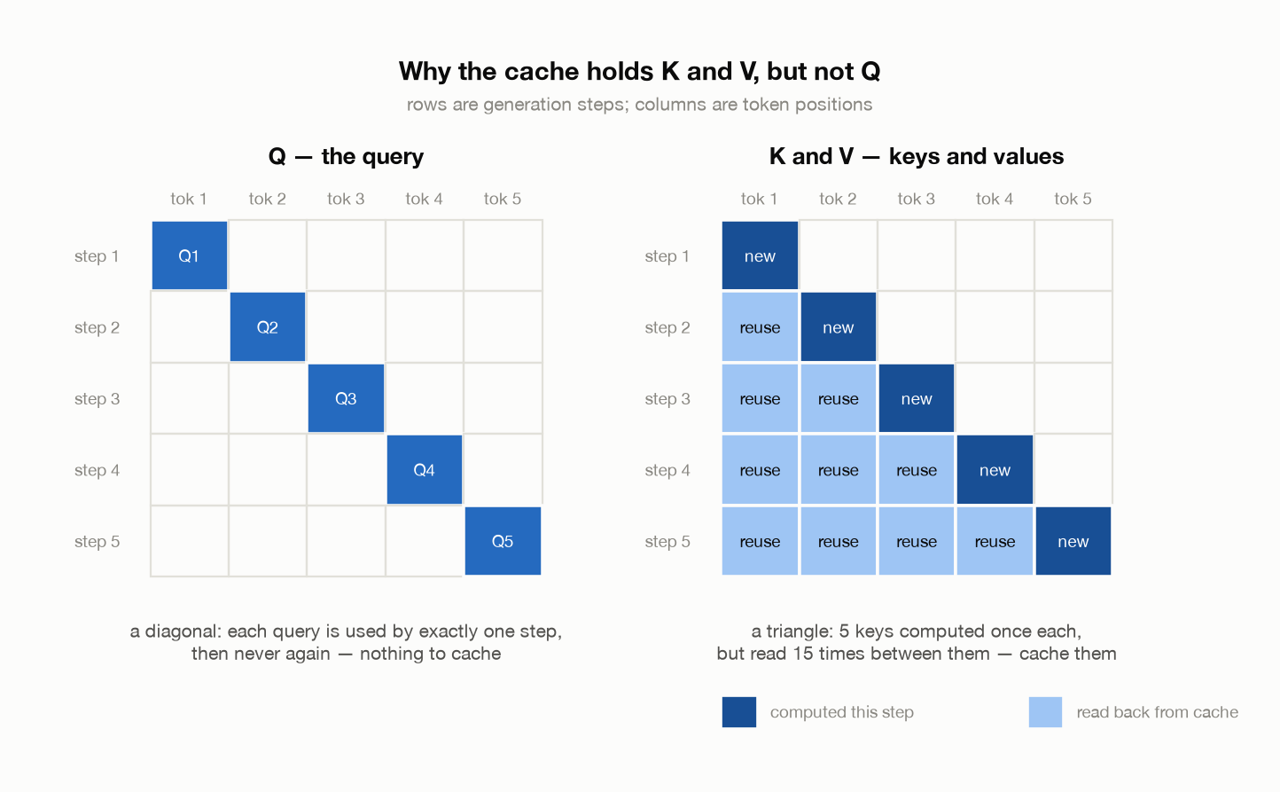
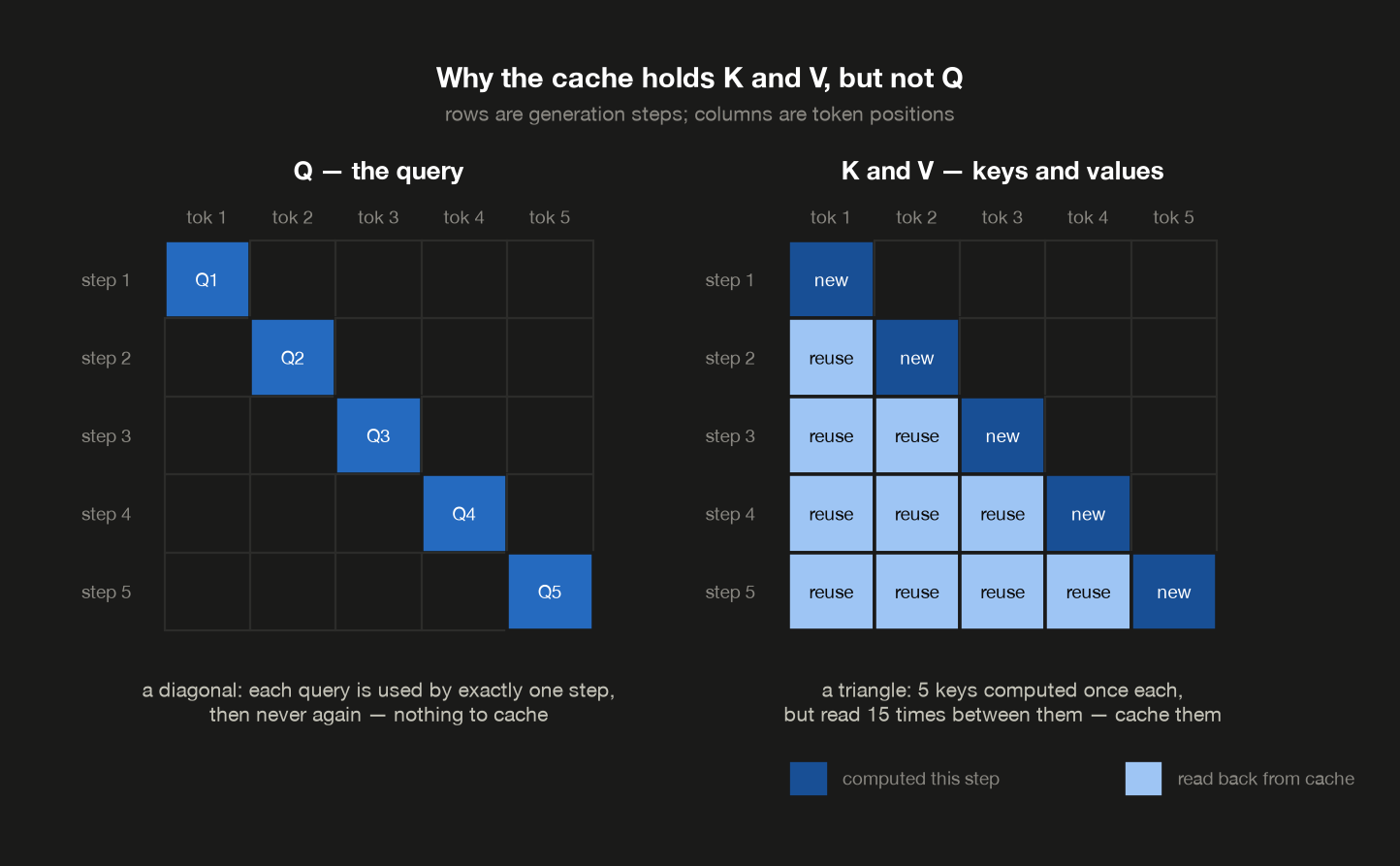
The shapes are the whole argument.
$Q$ fills a diagonal. Step 3 computes $Q_3$, uses it to produce token 4, and is then done with it — no later step ever asks for $Q_3$ again. A diagonal has nothing to reuse, so there is nothing a cache could save you.
$K$ and $V$ fill a triangle. Step 3 needs $K_1, K_2, K_3$; step 4 needs those plus $K_4$; step 5 needs all five. Every column extends downward forever. Across five steps, five keys get computed once each but read fifteen times between them — and by the arithmetic in the next section, that gap widens quadratically.
(That fifteen is a different count from the twelve above, and the difference is only the starting point: the figure walks five steps out from a single token, so the triangle is $1+2+3+4+5 = 15$, while the table earlier started from a three-token prompt and covered three steps, $3+4+5 = 12$. Same shape, sliced at different places. Whatever the prompt, the triangle grows as the square of the sequence and the diagonal grows linearly, which is the only part that matters.)
So the rule is not “keys and values are special”. It’s simply: cache what gets read again. In the diagram, that’s everything below the diagonal.
The same thing said as a table:
1
2
3
4
5
  tensor  cached?                                                   why
  -----------------------------------------------------------------------
  K           yes                   every later query scores against it
  V           yes                         every later query averages it
  Q            no  position i's query is used at step i and never again
$K_3$ and $V_3$ get read at step 3, and again at step 4, and at every step after. $Q_3$ is used once — to produce token 4 — and is then dead. Storing it would cost memory and save nothing.
This is also the answer to a question post 1 raised and left hanging: why does grouped-query attention shrink $K$ and $V$ but leave $Q$ at full width? Because $K$ and $V$ are what you have to keep. $Q$ is recomputed from scratch every step regardless.
The cache itself
So: compute $K$ and $V$ for exactly one new token per step, append them, and attend over everything stored.
1
2
3
4
5
6
7
8
9
10
11
class KVCache:
    def __init__(self, cfg, batch, device, dtype):
        shape = (cfg.n_layers, batch, cfg.n_kv_heads, cfg.max_seq_len, cfg.head_dim)
        self.k = torch.zeros(shape, device=device, dtype=dtype)
        self.v = torch.zeros(shape, device=device, dtype=dtype)

    def append(self, layer, k, v, start):
        end = start + k.shape[-2]
        self.k[layer, :, :, start:end] = k
        self.v[layer, :, :, start:end] = v
        return self.k[layer, :, :, :end], self.v[layer, :, :, :end]
Two details in that code are worth pausing on.
It’s pre-allocated to max_seq_len, not grown per step. Growing would reallocate and copy the whole cache every token. The price is that every sequence reserves its worst case up front whether it needs it or not — which is the fragmentation problem PagedAttention was built to solve.
RoPE is applied before K goes into the cache. Cached keys carry their rotation permanently, and you never re-rotate one as the sequence grows. That’s the point: position 3 stays position 3. Getting this wrong — re-rotating cached keys, or rotating a new token as though it were at position 0 — is the most common way to break a cache implementation.
2. The cache changes nothing about the output
Before optimizing anything, verify that it changes nothing. The model can generate either way, so run both on the same prompt and compare the tokens that come out:
1
2
3
4
with_cache = model.generate(prompt, max_new_tokens=24, use_cache=True)
without    = model.generate(prompt, max_new_tokens=24, use_cache=False)

torch.equal(with_cache, without)
1
2
3
4
  generated shape                    (2, 40)
  token ids identical                yes
  first 8 new tokens (cached)        [228, 432, 131, 158, 24, 111, 281, 506]
  first 8 new tokens (uncached)      [228, 432, 131, 158, 24, 111, 281, 506]
Identical token ids. This is the same category of claim as post 1’s check against the fused kernel, and it’s worth stating plainly because it’s the thing people get uneasy about: the KV cache is memoization, not approximation — it hands back numbers it already worked out, rather than estimating them. If your cached and uncached outputs diverge, you have a bug — most often a position-offset error where the new token is rotated as though it were at position 0.
3. Without a cache, generation is quadratic
Now the cost. Before the numbers, what “with and without the cache” actually means, because the entire experiment is one branch inside the generation loop:
1
2
3
4
5
6
7
8
9
for _ in range(max_new_tokens):
    next_token = logits[:, -1].argmax(-1, keepdim=True)   # greedy: take the top token
    idx = torch.cat([idx, next_token], dim=1)             # append it to the sequence

    if use_cache:
        logits = self(next_token, start=pos, cache=cache)  # one token, against the stored prefix
        pos += 1
    else:
        logits = self(idx, start=0, cache=None)            # the whole sequence, from scratch
Read the two calls. The cached path hands the model one token and points it at a cache holding everything before it. The uncached path hands over the entire sequence so far, every step, and computes every key and value again from position 0. Everything else — same weights, same greedy argmax, same tokens out — is identical, which is what §2 just checked. The only variable is how much work each step is asked to redo.
Then time both at growing output lengths, from a deliberately short prompt:
1
2
3
4
5
6
prompt_len = 64                       # short on purpose — see the note at the end
prompt = torch.randint(0, cfg.vocab_size, (1, prompt_len))

for n_new in (64, 128, 256, 512):
    cached   = benchmark_ms(lambda: model.generate(prompt, n_new, use_cache=True))
    uncached = benchmark_ms(lambda: model.generate(prompt, n_new, use_cache=False))
benchmark_ms warms up, synchronizes the GPU, then takes the median of several runs — a median rather than an average, so one scheduling hiccup on a laptop can’t move a row. That produces:
1
2
3
4
5
6
7
8
9
10
11
12
13
14
  prompt: 64 tokens; model: 7.8M params

  tokens generated  cached (ms)  uncached (ms)  speedup
  -------------------------------------------------------
  64                    53.2800        97.3100    1.83x
  128                   90.7372       227.4362    2.51x
  256                  148.4558       611.9815    4.12x
  512                  302.6207      1941.4126    6.42x

  8x more tokens costs (cached)      5.7x
  8x more tokens costs (uncached)    20.0x
  tokens processed at n=512 (cached) 576
  tokens processed at n=512 (uncached) 163584
  wasted work multiplier             284x
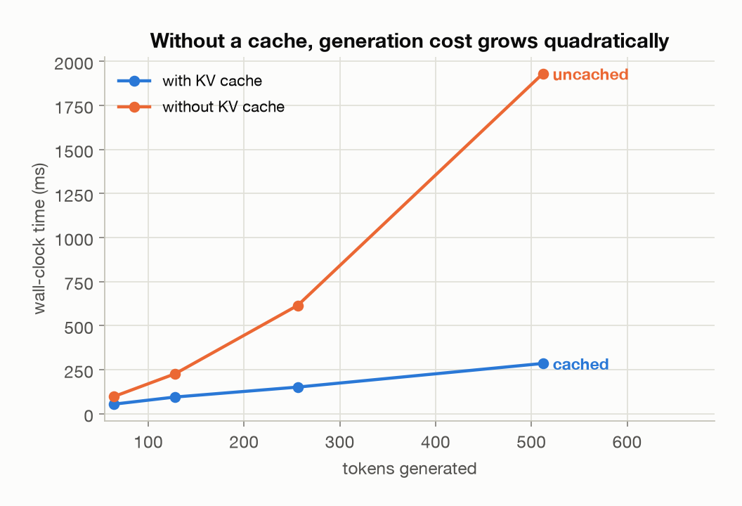
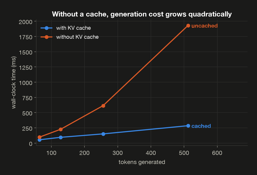
The two growth lines are the four rows divided end to end — 512 tokens against 64, hence “8× more tokens”:
1
2
growth_cached   = rows[-1]["cached_ms"]   / rows[0]["cached_ms"]     # 302.62 / 53.28
growth_uncached = rows[-1]["uncached_ms"] / rows[0]["uncached_ms"]   # 1941.41 / 97.31
8× the output costs roughly 5–6× with a cache and about 20× without. Wall-clock numbers wobble between runs, so don’t read the digits too closely; the contrast between “grows a bit faster than linear” and “grows like the square” is the part that holds.
The bottom three lines aren’t measurements
They’re counted, and the distinction matters — it’s the difference between a claim about my laptop and a claim about the algorithm. Nothing here is timed:
1
naive_tokens = sum(prompt_len + i for i in range(n_new))   # 64+0, 64+1, ... 64+511
Step $i$ of the uncached path re-processes all $64 + i$ tokens before it, so add those up across every step. To produce 512 tokens the cached path pushes $64 + 512 = 576$ tokens through the model — each one embedded exactly once. The uncached path pushes:
\[\sum_{i=0}^{511} (64 + i) \;=\; \underbrace{512 \times 64}_{32{,}768} + \underbrace{\frac{511 \times 512}{2}}_{130{,}816} \;=\; \mathbf{163{,}584}\]which is a 284× multiplier of pure repeated work. In general, for a prompt of $p$ tokens and $n$ generated:
\[\sum_{i=0}^{n-1} (p + i) \;=\; np + \frac{n(n-1)}{2}\]The first term is linear in what you generate; the second is the one that hurts. That is the whole claim of this section, and because it’s arithmetic rather than a benchmark, it comes out the same on your machine as on mine — the four timing columns will not.
One honest note about this measurement. I used a short prompt on purpose. With a long prompt the $np$ term dominates at these values of $n$ and the curve looks straight — you’d still see a big absolute saving, but not the shape. A short prompt isolates the $n^2/2$ term. Real serving has both: long prompts and long generations.
4. How big does the cache actually get?
First, what is physically in there. The cache stores computed numbers, not weights — and that distinction matters, because the two are different kinds of thing:
| Model weights | KV cache | |
|---|---|---|
| What it is | the learned parameters | K and V vectors computed from your tokens |
| Where it comes from | training | running the model on this conversation |
| Size | fixed | grows with every token |
| Shared between users? | yes, one copy serves everyone | no, every sequence has its own |
So they aren’t competing for the same reason. The weights are a one-time cost you pay to load the model. The cache is a running cost you pay per conversation, per token.
What one token costs
Concretely: for every token, at every layer, each key/value head stores one key vector and one value vector. Nothing else — no queries, no attention weights, no FFN activations. For Llama-3-8B in fp16:
1
2
3
4
5
6
7
  what                      count   running total
  -------------------------------------------------
  one key vector      128 numbers             128
  + one value vector  128 numbers             256
  x 8 KV heads                              2,048
  x 32 layers                      65,536 numbers
  x 2 bytes (fp16)                        128 KiB
One token of context costs 128 KiB. That’s the number worth remembering — everything else is multiplication.
(One label to be precise about: the layer shapes above are Llama-3-8B’s, but its own context window is 8k. The 128k figures throughout this post are Llama-3.1-8B, which has the identical layer shapes and differs only in how far the context extends. The per-token cost is the same either way; only how many tokens you can accumulate changes.)
And you pay it for every token in the conversation, not just the new one: the prompt you sent, the reply so far, all of it, for as long as the conversation lives.
1
2
3
4
5
  context         x KiB/token  cache (batch 1)
  ----------------------------------------------
  8,192 tokens        128 KiB         1.00 GiB
  32,768 tokens       128 KiB         4.00 GiB
  131,072 tokens      128 KiB        16.00 GiB
That walk up from one token is the formula. Here it is in one line, with its symbols first, in the order they appear:
| Symbol | What it is | Llama-3-8B |
|---|---|---|
| $L$ | how many blocks are stacked | 32 |
| $H_{kv}$ | key/value heads per block | 8 |
| $d_{head}$ | numbers in one key or value vector | 128 |
| $S$ | tokens in the sequence so far | grows every step |
| $B$ | sequences being served at once | your batch size |
The leading 2 is there because every position stores a key and a value. Everything else is a count of how many of those you end up holding.
Note which two are in there: sequence length $S$ and batch size $B$, both linear. The weights have neither — that difference is what the rest of this section is about.
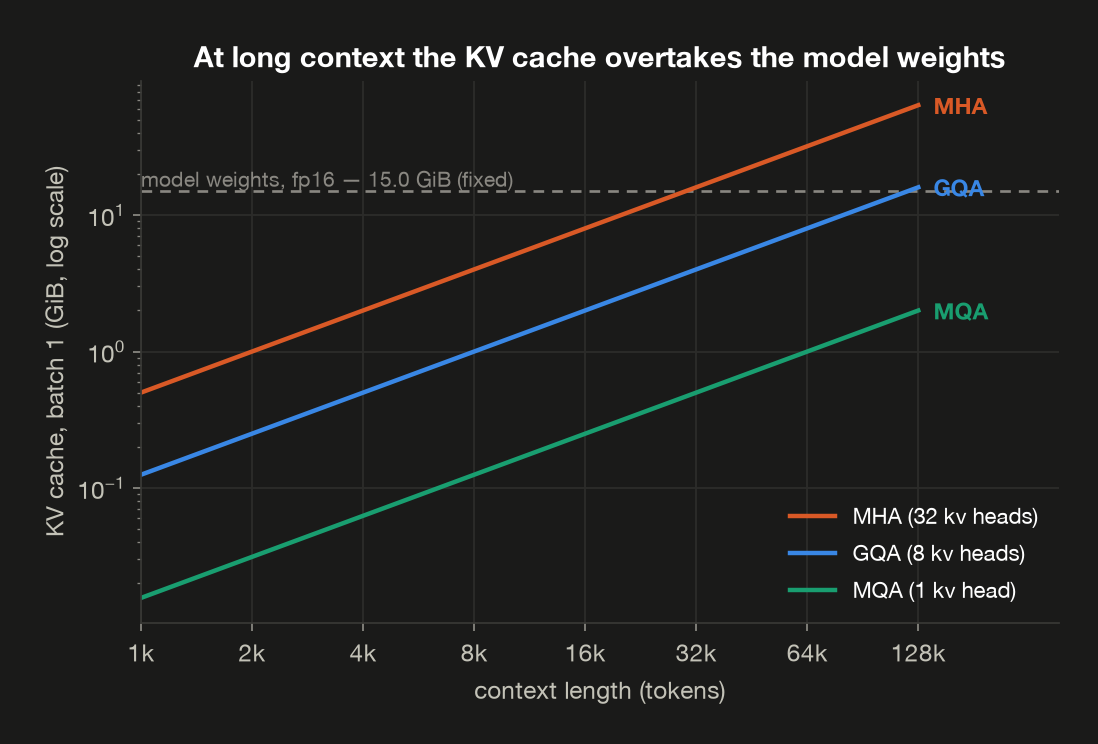
Llama-3-8B shapes, fp16, batch 1 — the weights are 15.0 GiB. The three rows are the three ways a model can allocate key/value heads: one per query head (MHA, multi-head attention), eight shared across 32 (GQA, grouped-query attention — what Llama-3-8B actually does), or a single one for all of them (MQA, multi-query attention). §5 covers what each costs you.
1
2
3
4
5
  variant           kv heads    4k ctx    8k ctx    32k ctx   128k ctx
  ----------------------------------------------------------------------
  as MHA                  32  2.00 GiB  4.00 GiB  16.00 GiB  64.00 GiB
  Llama-3-8B (GQA)         8  0.50 GiB  1.00 GiB   4.00 GiB  16.00 GiB
  as MQA                   1  0.06 GiB  0.12 GiB   0.50 GiB   2.00 GiB
So caching costs memory?
Yes — and it’s worth being explicit about that, because everything so far has made the cache sound like free money. It isn’t. It’s a time-memory trade.
Without a cache you still compute exactly the same keys and values every step. You just throw them away immediately, so they exist only while that layer is running — one layer’s worth at a time, then freed. The cache keeps all of them, for all 32 layers, alive for the whole conversation.
But the keys and values are not the largest thing the uncached path holds. Recomputing them means running all 131,072 tokens back through each layer, and that pass needs working memory of its own. Its largest moment is the FFN, whose gate and up projections each produce 14,336 numbers for every token, and both have to exist at once to be multiplied together:
1
2
3
4
5
6
7
8
  approach                 memory held                 made of
  --------------------------------------------------------------
  with a cache               16.00 GiB    K/V, 32 layers, kept
  without: attention step     3.50 GiB  residual, Q, K, V, out
  without: FFN step           8.00 GiB      residual, gate, up

  peak without a cache, at least     8.00 GiB
  memory held, cached vs not         at most 2.0x
Each row is 131,072 tokens × a width × 2 bytes. The FFN step is the residual stream (4,096 wide, 1.00 GiB) plus the gate and up outputs (14,336 wide, 3.50 GiB each), 8.00 GiB in all. The attention step, which holds the residual stream, the queries, the keys, the values and attention’s output, comes to 3.50 GiB. 8.00 GiB is a floor rather than a peak: it counts only tensors that every implementation must hold at the same moment, so a real run holds at least that much, whatever else it stores. That puts the cache at at most 2.0× the memory of recomputing.
Correction (2026-09-12). An earlier version of this section reported 10.7×. It counted the uncached path as one layer’s keys and values plus its hidden states, 1.50 GiB, and left out the FFN’s working memory, which is the largest thing that path holds.
The ratio is smaller than it first looks, but the two sides differ in a way the ratio hides: the uncached peak is a moment that comes and goes at every step, while the cache is held for as long as the conversation lives. What does holding it buy?
A request costs roughly in proportion to how many tokens the model has to push through itself. With a cache that’s the prompt and the reply, once. Without one, it’s the entire prefix again on every single step:
1
2
3
4
5
6
  prompt  reply  cached    uncached  compute saved
  --------------------------------------------------
  512       256     768     163,712           213x
  2,048     512   2,560   1,179,392           461x
  8,192   1,024   9,216   8,912,384           967x
  32,768  2,048  34,816  69,204,992          1988x
At most 2× the memory, for 200–2000× the compute. And the two sides scale differently: the memory cost grows linearly with context, while the compute saving grows quadratically. The longer the conversation, the better the bargain looks.
That’s why no serving stack ships without a KV cache. It isn’t a tuning option you enable for extra throughput — a 2,048-token prompt with a 512-token reply would cost 461× more to serve without it, which is the difference between a viable product and an impossible one.
That’s the honest framing for the rest of this section: the numbers below aren’t the cost of a mistake, they’re the price of a deliberate bargain. What makes them interesting is how quickly the price grows.
So at a 128k context, one conversation’s cache is 16 GiB — against 15 GiB for the entire model. One user’s scratch space outweighs the thing that took a fortune to train.
And that’s one user. Serving more doesn’t mean loading the model again — one copy of the weights answers everybody. But each concurrent conversation brings its own cache. So read the next table down the columns: the weights stay at 15.0 GiB no matter how many people you serve, while the cache multiplies by however many of them there are.
1
2
3
4
5
6
7
8
  model        batch    weights  KV cache @128k  cache/weights
  --------------------------------------------------------------
  Llama-3-8B       1   15.0 GiB        16.0 GiB          1.07x
  Llama-3-8B       8   15.0 GiB       128.0 GiB          8.56x
  Llama-3-8B      32   15.0 GiB       512.0 GiB         34.23x
  Llama-3-70B      1  131.5 GiB        40.0 GiB          0.30x
  Llama-3-70B      8  131.5 GiB       320.0 GiB          2.43x
  Llama-3-70B     32  131.5 GiB      1280.0 GiB          9.73x
That last row is worth doing by hand, because it’s the one that decides hardware budgets:
\[\underbrace{128\ \text{KiB}}_{\text{per token}} \times \underbrace{131{,}072}_{\text{tokens}} = \underbrace{16\ \text{GiB}}_{\text{one conversation}} \qquad 16\ \text{GiB} \times 32\ \text{users} = 512\ \text{GiB}\]Thirty-two concurrent conversations at 128k context need half a terabyte of KV cache — about six 80 GiB accelerators’ worth, for a model whose weights fit comfortably on one. This is why “how many users can I serve?” is a KV-cache question, not a model-size question, and why the answer changes completely with context length.
It’s also why the 70B row is interesting: at batch 1 its cache is only 0.30× its weights, so a big model at short context is weight-dominated, while a small model at long context is cache-dominated. Two very different engineering problems wearing the same “LLM inference” label.
5. Shrinking the cache: GQA, MQA, and what you give up
Notice that $H_{kv}$ — the number of key/value heads — is in the formula, but the number of query heads isn’t. That’s the lever.
- MHA: every query head gets its own K/V head. Maximum expressiveness, maximum cache.
- MQA: all query heads share a single K/V head. 32× smaller cache here, but a real quality cost — every head is forced to look up against the same keys. Shazeer proposed it in Fast Transformer Decoding (2019) for exactly this reason: decoding was already memory-bound.
- GQA: query heads are split into groups, one K/V head each. Llama-3-8B uses 8 KV heads for 32 query heads — 4× less cache than MHA at a quality cost small enough that it’s now the default. Ainslie et al., GQA (2023), also gave a recipe for uptraining an existing multi-head checkpoint into a grouped-query one for about 5% of the original pre-training compute — you didn’t have to retrain to adopt it, which is part of why it spread so fast.
In code the sharing is just a broadcast before the attention call:
1
2
3
if self.n_rep > 1:
    k = k.repeat_interleave(self.n_rep, dim=1)
    v = v.repeat_interleave(self.n_rep, dim=1)
The expansion happens after the cache read, which is the entire point: you store 8 heads and compute against 32.
What that actually buys, measured
That’s two claims — the cache shrinks, the computation doesn’t — so here they are side by side. Same model built three times, 12 query heads throughout, only n_kv_heads changing:
1
2
3
4
5
  variant  kv heads  q per kv  params  cache @512       vs MHA  ms/decode step
  ------------------------------------------------------------------------------
  MHA            12         1   68.9M    24.0 MiB            —          4.5366
  GQA             4         3   62.6M     8.0 MiB   3x smaller          5.9625
  MQA             1        12   60.3M     2.0 MiB  12x smaller          5.1851
Compare the two right-hand columns. The cache column tracks n_kv_heads exactly — 24 → 8 → 2 MiB, a 12× swing, with no approximation anywhere in it. The time column stays inside a 1.3× band. That gap is why GQA caught on: it is a storage decision that the compute side barely notices. (The toy shares 3 query heads per KV head where Llama-3-8B shares 4; the ratio is whatever n_kv_heads says it is.)
Don’t read the ordering inside that time column, though. The three numbers sit close enough together that which one lands last shuffles between runs on this laptop — I’ve had GQA slowest and MQA slowest on consecutive runs. What holds every time is this: fewer K/V heads never bought a faster decode step. If anything it costs a little, and the repeat_interleave above is why. It allocates the widened tensor instead of viewing it, so work you took out of storage comes back at you as a copy. Production kernels read the shared K/V directly and never build that tensor; PyTorch exposes this as scaled_dot_product_attention’s enable_gqa flag.
So, the caution to take away: “the cache got smaller” and “the kernel got faster” are separate claims, and this table only earns the first.
Post 12 covers DeepSeek’s MLA, which attacks the same problem differently — compressing K and V into a shared low-rank latent and caching that instead.
6. Prefill vs decode: the whole ballgame
Generation has two phases with completely different performance characteristics.
Prefill processes the entire prompt in one parallel pass. Decode produces one token per pass. In code the only difference is how many tokens go in — the model, the weights and the cache are the same:
1
2
3
4
5
# prefill: the whole 512-token prompt at once, into an empty cache
model(prompt, start=0, cache=cache)          # prompt is (1, 512)

# decode: one token, against a cache that already holds 512
model(one_token, start=512, cache=cache)     # one_token is (1, 1)
Timing both on the same 62.6M-parameter model:
1
2
3
4
5
6
  phase    tokens/pass  ms/pass  ms/token    tokens/s
  -----------------------------------------------------
  prefill          512  33.6026    0.0656  15236.9235
  decode             1   5.4777    5.4777    182.5581

  per-token cost, decode / prefill   83.5x
A token costs roughly two orders of magnitude more to generate than to read. Both passes stream the same weights through the chip’s arithmetic units (ALUs — the circuits that actually do the multiplying). Prefill amortizes that read across 512 tokens; decode pays it in full for one.
The exact multiple is the least trustworthy number in this post. Across repeated runs on this laptop it lands anywhere between about 80× and 100×, depending on what else the machine is busy with. The order of magnitude is what holds, and it is the only part the argument needs.
The clean way to see why is arithmetic intensity — FLOPs performed per byte of weights moved:
1
2
3
4
  phase    tokens  FLOPs (2*N*P)  weight bytes  FLOP/byte
  ---------------------------------------------------------
  prefill     512         64.1 G      0.23 GiB   256.0000
  decode        1        0.125 G      0.23 GiB     0.5000
Where “100–300 FLOP/byte” comes from
That threshold gets quoted a lot, usually with no source attached, so let’s not leave it as folklore. It isn’t really a rule of thumb at all — it’s a property of the chip, and you can divide it out yourself.
Think about the two ceilings any kernel runs into. One is arithmetic: the chip can only perform so many multiplies per second. The other is memory: it can only fetch so many bytes per second out of HBM, the bank of high-bandwidth memory sitting beside the processor — the “80 GB” a spec sheet quotes. Which ceiling you hit depends on how much arithmetic you do per byte you fetch. Do very little, and you spend your time waiting for bytes. Do a lot, and the bytes keep up and the multipliers become the limit.
Plot achievable speed against arithmetic-per-byte and you get a line that climbs while memory is the constraint, then goes flat once arithmetic is. That shape is the roofline, and the corner where it flattens is the ridge point — the arithmetic-per-byte at which the two ceilings meet. It sits at exactly peak throughput divided by bandwidth. Below the ridge, no kernel can keep the arithmetic units busy however well it’s written, because the bytes cannot arrive fast enough to feed them.
Drawn, with this post’s two phases placed on it:
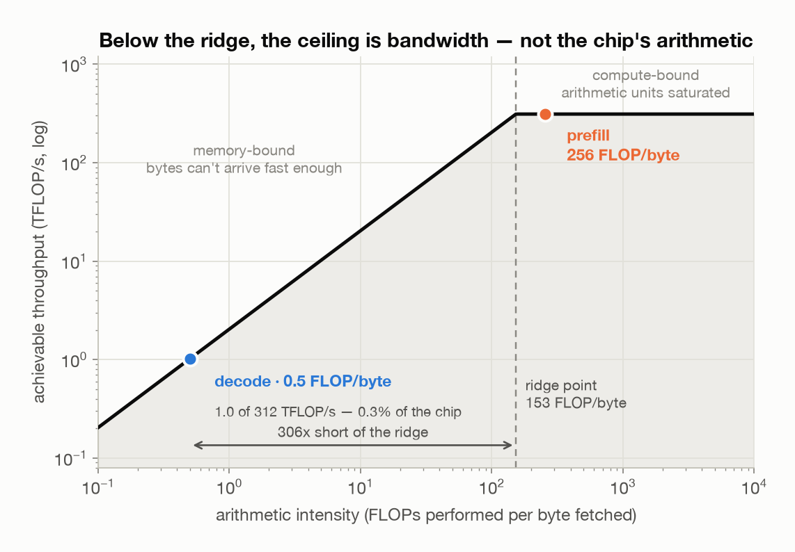
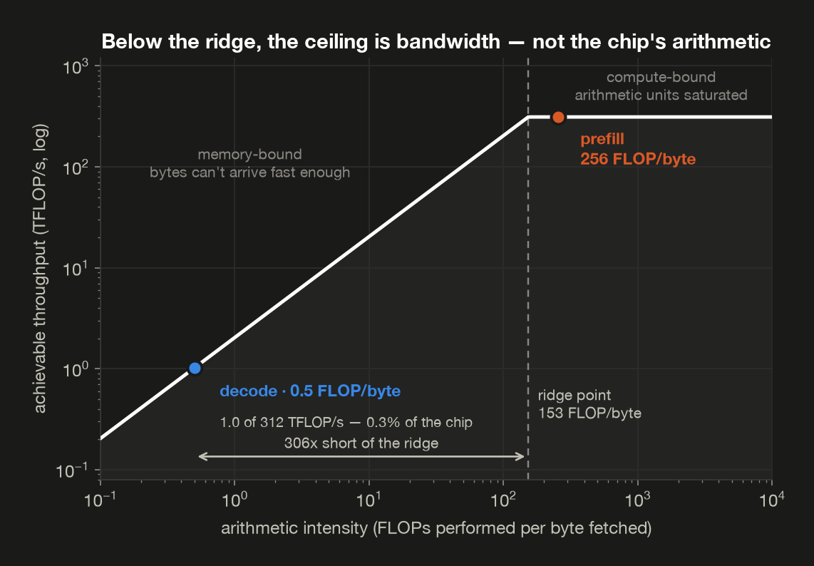
Both dots sit on the roof, and that placement is the point. A memory-bound kernel isn’t failing to reach its ceiling — the sloped stretch is its ceiling. Decode is doing as well as it possibly can, and as well as it possibly can is 1.0 of the chip’s 312 TFLOP/s. Prefill, one flat stretch away, gets all 312.
Note also what the picture makes obvious and the numbers hide: 0.5 and 256 look like “small and large” written down, but on the axis they are three orders of magnitude apart, and the corner sits between them.
So divide one datasheet number by the other and you have it:
1
2
3
4
5
6
7
8
  accelerator     dense fp16  HBM bandwidth    ridge point
  ----------------------------------------------------------
  A100 40GB SXM  312 TFLOP/s     1,555 GB/s  201 FLOP/byte
  A100 80GB SXM  312 TFLOP/s     2,039 GB/s  153 FLOP/byte
  H100 SXM       989 TFLOP/s     3,350 GB/s  295 FLOP/byte
  H200 SXM       989 TFLOP/s     4,800 GB/s  206 FLOP/byte

  ridge point, across these four     153-295 FLOP/byte
These are vendor peak figures, not anything I measured — the one table here that comes off a spec sheet rather than out of my laptop, and labelled as such. But look at how little the spread moves: 153 to 295, across two architectures and a 3× jump in raw FLOP/s. Bandwidth and arithmetic have grown closely enough in step that the ridge stayed put, which is why a rule of thumb this crude has outlived the hardware it was coined for. Notice too that H100 → H200 buys bandwidth at identical FLOP/s, and so lowers the ridge — more workloads end up on the compute-bound side of it.
Now place the two phases against the narrowest of those ridges:
1
2
3
4
5
6
  phase    FLOP/byte  vs ridge (153)                      verdict
  -----------------------------------------------------------------
  prefill      256.0           1.67x  at or above — compute-bound
  decode         0.5         0.0033x  far below — bandwidth-bound

  decode is short of the ridge by    306x
Prefill sits at 256 — past the ridge on the two A100s, near it on the Hopper parts, comfortably in the productive zone either way. Decode sits at 0.5, short of the easiest ridge by 306×. The hardware spends essentially all of decode waiting on memory. It is memory-bandwidth-bound.
And that’s a statement about the workload, not the implementation. There is no kernel that fixes a 306× shortfall — you have to change the arithmetic-per-byte ratio itself, which is exactly what every optimization below does. Pope et al., Efficiently Scaling Transformer Inference (2022), work the same analysis through at production scale if you want it in more depth than one table.
This single fact explains a startling amount:
- Batching works — the weight read is already paid for, so more sequences are nearly free (until they aren’t; see below).
- Quantization speeds up decode even when the arithmetic isn’t faster, because there are simply fewer bytes to move.
- Speculative decoding wins because verifying $k$ draft tokens in one pass costs about the same as generating one — you were bandwidth-bound, not compute-bound.
- Bigger GPUs don’t help decode much unless their bandwidth went up.
The same asymmetry, on an invoice
Everything above is measured on my laptop, which is a fine way to see a mechanism and a poor way to believe it matters. So here is the same split priced by someone who serves this workload for a living. Every major LLM API bills input tokens and output tokens at different rates, and those are exactly our two phases: input tokens are the ones you prefill, output tokens are the ones you decode.
Claude’s published rates, per million tokens:
| Model | Input | Output | Output ÷ input |
|---|---|---|---|
| Claude Haiku 4.5 | $1 | $5 | 5× |
| Claude Sonnet 5 | $3 | $15 | 5× |
| Claude Opus 5 | $5 | $25 | 5× |
| Claude Fable 5 | $10 | $50 | 5× |
Read the last column. A tenfold spread in price from the cheapest model to the most capable, and the ratio never moves. Whatever else changes between a small model and a large one, the fact that a generated token costs more than a read one — and by how much — does not. That’s the shape of the workload, not a property of any one model, which is exactly what §6 has been arguing from the FLOP/byte side.
Now the honest part, because 5× is not 83×. My measurement was one sequence with the whole machine to itself, and §7 is about to show what changes when it isn’t. Batching amortizes the weight read across many concurrent users — and the weight read is precisely what makes decode expensive. Divide the unbatched 83× by the 16× throughput gain §7 measures at batch 32 and you land near 5. I’d treat that as the right order of magnitude rather than a derivation: published prices reflect hardware, utilization, competition, and margin, not a cost pass-through, and no vendor owes us the arithmetic. What transfers is the direction. Decode costs more, output tokens cost more, and the gap on the invoice is much narrower than the gap on my laptop because production serving does the one thing my measurement didn’t — it batches.
And the cache itself is a line item
The API also sells you the thing this whole post is about. Prompt caching reuses the computed state of a prompt prefix across requests, so a conversation’s shared preamble is prefilled once rather than on every turn:
| Multiple of the base input rate | |
|---|---|
| Cache read | ~0.1× |
| Cache write, 5-minute lifetime | 1.25× |
| Cache write, 1-hour lifetime | 2× |
Reading back a prefix costs about a tenth of computing it — pay 1.25× once, then 0.1× forever after, so the 5-minute tier breaks even on the second request — 1.25 + 0.1 = 1.35 against the 2.0 you’d pay for two uncached passes. That is §4’s time-memory trade with the memory side rented rather than owned, and it prices the cache-versus-recompute question we’ve been answering in milliseconds.
The rule governing what you can cache is where this gets satisfying, because we derived it back in §1 without knowing it had a price attached. Caching is a prefix match: change one byte anywhere in the prompt, and everything from that byte onward is invalidated — while everything before it stays valid and stays cheap.
That is causal masking, sold by the token. A token cannot influence anything that came before it, so an edit at position $N$ leaves positions $1 \ldots N-1$ untouched and their keys and values still correct. It can influence everything after it, so positions past $N$ must be built again. The same two facts that made a KV cache sound in §1 are what make a prompt cache billable here — which is also why the practical advice for keeping costs down (“put your stable system prompt first, put the volatile per-request bits last”) isn’t a vendor quirk. It’s the triangle from §1, arranged so the reusable part comes first.
7. The batch sweep, and where it stops working
First, what a batch is, since everything below turns on it. A batch is a set of separate, unrelated conversations that the model runs through in the same forward pass. “Batch 32” means thirty-two different users, each part-way through their own conversation, each about to be handed their next token — not thirty-two tokens of one conversation. The batch axis runs across users; sequence length is the other axis entirely, and you can see both sitting in the cache shape from §1:
1
2
3
(n_layers, batch, n_kv_heads, max_seq_len, head_dim)
#           ↑                      ↑
#     how many conversations   how long each one is
Every batch slot carries its own private cache. Hold that thought — it’s the whole of what happens later in this section.
(In training the word means something related but different: many examples per gradient update. Here there is no gradient. A batch is just independent users sharing one trip through the weights.)
Why share a trip at all? Think of the weights as a large reference book. To produce even a single token, the model has to pull the whole book out of memory and through the chip — that read is the cost of decoding, which is what §6 just established. Read it for one waiting user and you get one token out of it. Read it with thirty-two users waiting and you answer all thirty-two on the way through, for a read that was going to happen regardless.
So if decode is really memory-bound, batching should buy throughput almost for free. The sweep fills a cache for batch sequences, then times a single decode step across all of them at once:
1
2
3
4
5
6
for batch in (1, 2, 4, 8, 16, 32):
    cache = KVCache(cfg, batch, device, dtype)
    model(warm, start=0, cache=cache)        # warm is (batch, prefix)

    step = torch.randint(0, cfg.vocab_size, (batch, 1))   # one token per sequence
    ms = benchmark_ms(lambda: model(step, start=prefix, cache=cache))
With a short (32-token) prefix:
1
2
3
4
5
6
7
8
  batch  ms/step  latency vs b=1  tokens/s  throughput vs b=1
  -------------------------------------------------------------
  1       4.0566           1.00x       247               1.0x
  2       4.2638           1.05x       469               1.9x
  4       5.1109           1.26x       783               3.2x
  8       5.7412           1.42x      1393               5.7x
  16      6.6779           1.65x      2396               9.7x
  32      8.0730           1.99x      3964              16.1x
32× the work for 1.99× the time — 16.1× the throughput. The GPU was idling on memory, so the extra sequences rode along inside a weight read that was happening anyway. That is what memory-bound looks like, and it’s why every serving stack batches aggressively.
Read the two ratio columns against each other before moving on, because they are measuring opposite things and the gap between them is the deal you’re making. Latency went up 1.99×: every one of those users now waits about twice as long for each token as they would with the machine to themselves. Throughput went up 16.1×: you are producing sixteen times more text per second across all of them.
Batching makes nothing faster for anybody. It makes the machine far more productive, and each individual user pays for that in patience. You take the trade because you are serving thirty-two people with it instead of one — and it’s why picking a batch size is a scheduling decision about who waits how long, not a throughput setting you turn up.
Now the same sweep with a 512-token prefix:
1
2
3
4
5
6
7
8
  batch  ms/step  latency vs b=1  tokens/s  throughput vs b=1
  -------------------------------------------------------------
  1       5.3091           1.00x       188               1.0x
  2       7.1850           1.35x       278               1.5x
  4       9.0274           1.70x       443               2.4x
  8      14.2632           2.69x       561               3.0x
  16     22.6502           4.27x       706               3.8x
  32     39.7221           7.48x       806               4.3x
The free lunch is gone: 16.1× throughput becomes 4.3×.
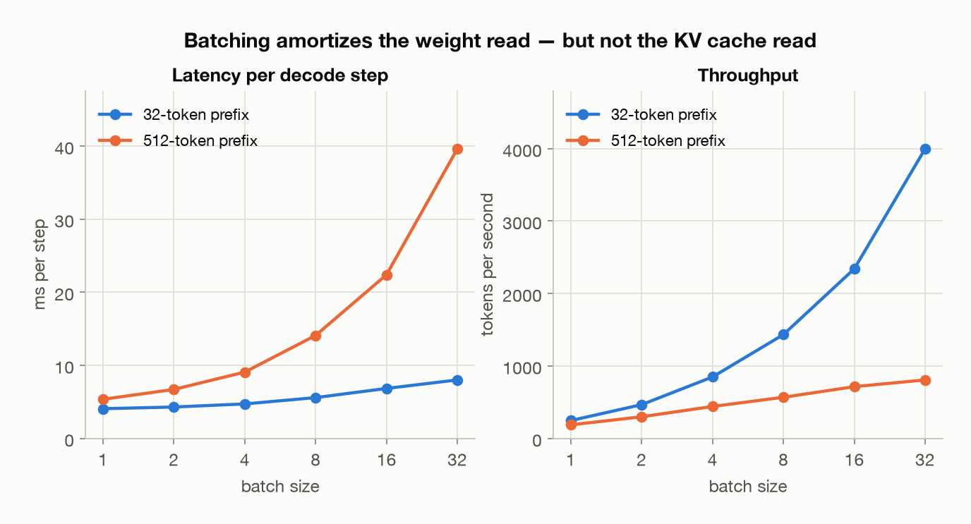
The reason is the formula from §4. Weights are shared across the batch; the KV cache is not. Every sequence brings its own cache, so KV traffic scales with batch while weight traffic stays flat.
Back to the reference book. Alongside it, each user has a notebook of their own — their KV cache — and the model has to read that too. With one user the notebook is nothing next to the book, so sharing the book is nearly the whole cost and extra readers are nearly free. But notebooks don’t get shared. Thirty-two users bring thirty-two notebooks, and at some point you are spending longer on notebooks than on the book, whereupon another reader is no bargain at all.
That’s a claim about two numbers, so here are the two numbers, per decode step, at the 512-token prefix:
1
2
3
4
5
6
7
8
9
10
11
  batch  weight bytes   KV bytes      total  KV share  bound by
  ---------------------------------------------------------------
  1         0.233 GiB  0.008 GiB  0.241 GiB        3%   weights
  2         0.233 GiB  0.016 GiB  0.249 GiB        6%   weights
  4         0.233 GiB  0.031 GiB  0.265 GiB       12%   weights
  8         0.233 GiB  0.062 GiB  0.296 GiB       21%   weights
  16        0.233 GiB  0.125 GiB  0.358 GiB       35%   weights
  32        0.233 GiB  0.250 GiB  0.483 GiB       52%  KV cache

  KV overtakes weights at batch (32-tok prefix) 478
  KV overtakes weights at batch (512-tok prefix) 30
Two lines and where they cross, drawn:
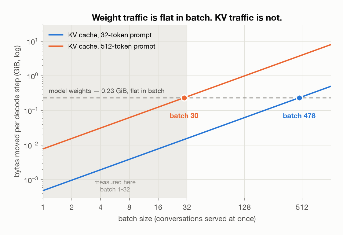
The weight line is horizontal because one copy of the weights serves everybody. The KV lines are diagonal because every conversation brings its own cache. Everything in this section is those two facts and the point where the diagonal overtakes the horizontal.
And the shaded band explains the two sweeps above. With a 512-token prompt the crossing is at batch 30 — inside the range I measured, which is exactly why that sweep flattened out in front of us. With a 32-token prompt it’s at batch 478, far off the right of anything I ran, which is why that sweep still looked like a free lunch all the way to 32. Same model, same hardware, same argument; sixteen times the context moves the crossing sixteen times earlier.
Read the weight column: it never changes. Read the KV column: it doubles every row. Somewhere between batch 16 and 32 they cross, and the KV share goes from a rounding error at 3% to the majority of memory traffic at 52%.
Line that up against the throughput column above and the two tell one story. Throughput is still climbing steeply while KV share is under 20%; it flattens as the share passes half. Batching amortizes one term and multiplies the other, and the shape of the curve is just which term is winning.
The last two rows are the same crossover stated as a batch size, and the gap between them is the point: with a 32-token prefix you’d need batch 478 before the cache matters, with a 512-token prefix you need batch 30. Sixteen times the context, sixteen times sooner. The context length you support and the batch size you can profitably run are the same decision.
I find this the most useful thing in the post, because the textbook version (“decode is memory-bound, so batch it”) is only half the story. Batching amortizes one term. The other term grows with exactly the thing you were batching. That crossover is why production serving is a scheduling problem — continuous batching to refill a slot the moment any sequence finishes, rather than making everyone wait on the longest one; prefix sharing for common system prompts; paged caches to stop reserving worst-case memory; and KV-cache quantization to shrink the term that doesn’t amortize.
(These are laptop numbers on Apple Silicon with a small model, so the absolute values reflect a modest bandwidth budget and some kernel-launch overhead. The shape of both curves, and the crossover between them, is what transfers — that’s arithmetic, not hardware.)
But surely compute runs out too?
Everything above is bytes. Weight traffic, KV traffic — memory, both of them. Yet the model still has to do the matmuls, and every user you add is one more full pass through the weights. That work is shared with nobody. So why isn’t arithmetic the thing that runs out first?
It’s a fair objection, and the honest answer is that compute scales exactly the way KV traffic does. Per decode step at batch $B$:
1
2
3
4
5
  term                  scales as            shared across users?
  -----------------------------------------------------------------
  weight reads     15.0 GiB, flat  yes — one copy feeds everybody
  weight matmuls   2 x params x B      no — one pass per sequence
  KV cache reads  128 KiB x S x B     no — one cache per sequence
Batching amortizes the first and multiplies the other two. So the plateau above could be either of the unshared terms — bandwidth or arithmetic — and the sweep alone can’t tell you which.
Settle it by starting with attention over the cache, since that is the part doing the reading. Its FLOPs and its bytes both scale with $B$ and with $S$, so both cancel, and what’s left is a constant of the architecture:
\[\frac{\text{attention FLOPs}}{\text{KV bytes}} = \frac{4\,n_{heads}\,S\,d_{head}\,L}{2\,H_{kv}\,S\,d_{head}\,L \times \text{bytes}} = \frac{2\,n_{heads}}{H_{kv} \times \text{bytes}}\]In fp16 the bytes cancel too and that is simply $n_{heads} / H_{kv}$ — the grouping ratio, and nothing else:
1
2
3
4
5
  variant           kv heads  q heads per kv head  FLOP/byte
  ------------------------------------------------------------
  as MHA                  32                    1        1.0
  Llama-3-8B (GQA)         8                    4        4.0
  as MQA                   1                   32       32.0
Which hands §5 a second job I didn’t give it credit for. Sharing K/V heads doesn’t only shrink the cache — it raises the arithmetic intensity of every read from that cache by the very same factor. Four times less to store, four times more work done per byte stored.
Now put the two together and solve for the batch size at which the matmuls finally take longer than the bytes take to arrive:
1
2
3
4
  accelerator    ridge  S=128   S=1k   S=8k  S=32k
  --------------------------------------------------
  A100 80GB SXM    153    181  never  never  never
  H100 SXM         295    424  never  never  never
At a very short context the answer is a real batch size, and it lands suspiciously close to the ridge point. That’s not a coincidence: the weight term’s arithmetic intensity is $2B/\text{bytes}$, which in fp16 is just $B$, so it crosses the ridge at a batch equal to the ridge.
Past about a thousand tokens of context, the answer is never. The KV read sits at 4 FLOP/byte against a ridge of 153 — every user you add brings 38× more bytes than the hardware can pay for with arithmetic, so the gap widens rather than closes. No batch size climbs out of it.
So compute genuinely never amortizes, and it still isn’t what binds. At any context worth having, the cache read gets there first and stays there. Where arithmetic does bind is the other phase entirely: prefill is compute-bound from batch 1 (§6), which means your FLOPs ceiling governs how fast you can take on new conversations, while bandwidth and cache capacity govern how many you can carry. Two different limits, two different fixes, and a serving stack has to respect both.
(This one is arithmetic from model shapes and datasheet peaks, not a measurement — the same footing as the ridge-point table in §6, and for the same reason: my laptop cannot reach batch 181.)
8. A worked example: 1,000 users at 128k
Everything so far has been measured one piece at a time. Point all of it at a single question and see what comes out: you want to serve Llama-3.1-8B to a thousand people at once, each with the full 128k context. How much hardware is that?
Start where §4 left off. One token of context costs 128 KiB, a full 128k context costs 16 GiB, and a thousand of those is:
1
2
3
4
  what            per user      x 1,000 users
  ---------------------------------------------
  KV cache       16.00 GiB          15.62 TiB
  model weights          —  14.96 GiB per GPU
Fifteen and a half terabytes of scratch space, for a fifteen-gigabyte model. The weights are now a rounding error — you are not buying hardware to hold the model, you are buying it to hold the conversations. Divide that by what a card can actually give you:
1
2
3
4
5
  accelerator       HBM  usable for KV  users/GPU  GPUs needed  tok/s per user
  ------------------------------------------------------------------------------
  A100 80GB SXM   80 GB         50 GiB        3.1          320              29
  H100 SXM        80 GB         50 GiB        3.1          320              48
  H200 SXM       141 GB        101 GiB        6.3          159              38
Roughly 320 H100s — three users per card. Which is worth not taking on trust, since it’s the number that decides the budget.
Where those three columns come from
They’re three chained formulas, each feeding the next:
1
2
3
4
5
6
usable         = hbm * 0.90 - weight_bytes - 2 GiB   # what's left for cache
per_gpu        = usable / kv_per_user                # users/GPU
n_gpus         = ceil(total_users / per_gpu)         # GPUs needed
bytes_per_step = kv_per_user * per_gpu + weight_bytes
step_s         = bytes_per_step / bandwidth
tok_s_per_user = 1 / step_s                          # tok/s per user
Worked through for the H100 row:
1
2
3
4
5
6
7
8
  column                               arithmetic     result
  ------------------------------------------------------------
  usable for KV   74.51 GiB x 0.90 - 14.96 - 2.00  50.10 GiB
  users/GPU                         50.10 / 16.00      3.131
  GPUs needed                 ceil(1,000 / 3.131)        320
  bytes per step            16.00 x 3.131 + 14.96  65.06 GiB
  step time               65.06 GiB / 3,120 GiB/s   20.85 ms
  tok/s per user                     1 / 20.85 ms       48.0
The first row is a conversion and then three subtractions. Vendors quote capacity and bandwidth in decimal units, and everything this post computes is binary, so both get divided by $1024^3$ before they meet anything else:
\[\frac{80 \times 10^{9}\ \text{B}}{1024^3} = 74.51\ \text{GiB}, \qquad \frac{3{,}350 \times 10^{9}\ \text{B/s}}{1024^3} = 3{,}120\ \text{GiB/s}\]That is the whole of why the table says 74.51 where the box says 80, and 3,120 where the datasheet says 3,350. Mixing the two families is the classic way to land a plausible number nobody else can reproduce — subtract GiB from bytes and you are out by a factor of a billion; divide GiB by GB/s and the step time comes out 19.42 ms instead of 20.85.
Then the three subtractions: 90% is what a serving stack can actually reach once you allow for allocator overhead and fragmentation; 14.96 GiB is one copy of the weights, on every card; 2 GiB is activation working space. An 80 GB card is left with 50 GiB, and a single 128k conversation wants 16 of them.
The last three rows rest on two facts, and they’re the ones to hold onto:
- Every decode step re-reads each resident user’s entire cache. Attention at any step attends over every earlier position, so all 128k of them get read again, for every user, for every token. That’s the multiplication by
per_gpu— and it’s why the step is 65 GiB rather than 15. - One step emits one token for every resident user at once. So a single user sees
1/step— 48 tokens a second — while the card as a whole seesper_gpu/step, about 150. Per-user speed is a property of one card’s loop, not of the fleet: those 320 GPUs each run their own 20.85 ms cycle.
The last two columns answer different questions, and conflating them is how sizing goes wrong. Capacity sets the fleet size — the A100 and the H100 need the same 320 cards because they hold the same 80 GB. Bandwidth sets the token rate, and there the H100 is worth 1.6× the A100 for an identical bill of materials.
The H200 row is the one worth sitting with, and now the formulas make it legible. Twice the capacity halves the fleet, and each user gets slower:
1
2
3
4
  card             bytes per step           =    bandwidth      step  tok/s
  ---------------------------------------------------------------------------
  H100 SXM  16.00 x 3.131 + 14.96   65.06 GiB  3,120 GiB/s  20.85 ms     48
  H200 SXM  16.00 x 6.327 + 14.96  116.19 GiB  4,470 GiB/s  25.99 ms     38
Because per_gpu isn’t only an output of the first formula — it’s a multiplier inside the second. More resident users means more cache to re-read every step. Follow the four growth rates and the whole thing falls out:
1
2
3
4
  raw HBM, H100 -> H200              +76%
  usable for KV                      +102%
  bytes moved per step               +79%
  bandwidth                          +43%
Usable capacity outruns raw capacity (+102% against +76%), because the weights and the headroom come off once regardless of card size — a bigger card gives disproportionately more of its extra memory to cache. Bytes per step then lags usable capacity (+79%), because the weight read is shared across everyone on the card. And bandwidth grows slowest of all, at +43%.
That last mismatch is the whole story: 79% more to move, 43% more speed to move it with, so the step stretches from 20.85 ms to 25.99 ms. The H200 is better at everything and still hands each user fewer tokens per second. Capacity buys density; only bandwidth buys speed — and buying the first without the second makes every user wait longer.
Is it fast enough, and what is it doing?
1
2
3
4
5
6
  per decode step         bytes or time             share
  ---------------------------------------------------------
  KV cache read                50.1 GiB               77%
  weight read                  15.0 GiB               23%
  time, memory-bound            20.9 ms                 —
  time, if compute-bound        0.27 ms  1.3% of the step
Every decode step re-reads 50 GiB of cache against 15 GiB of weights. The term batching was supposed to amortize is now under a quarter of the traffic — §7’s crossover, arriving at production scale. And compute is 1.3% of the step: the “never” column from the section above, seen from the deployment end. You could triple the FLOPs of every card in that fleet and serve the same thousand users at the same speed.
What actually moves the number
1
2
3
4
5
6
  lever                             cache/user  users/GPU  H100 SXMs needed
  ---------------------------------------------------------------------------
  baseline — fp16 cache, full 128k   16.00 GiB        3.1               320
  quantize the KV cache to fp8        8.00 GiB        6.3               160
  cap context at 32k                  4.00 GiB       12.5                80
  both                                2.00 GiB       25.0                40
320 cards to 40, and not one of those levers touches the model or adds a single FLOP. Both of them shrink the cache — one by storing each number in half the space, the other by keeping fewer of them. That is the entire argument of this post arriving as a purchase order, and it is why “how long a context do we advertise?” is a hardware-budget decision wearing a product-spec costume.
(Analytic, like the ridge points in §6 — model shapes and datasheet capacities, not something a laptop can measure. The usable-memory assumption is deliberately generous; real serving stacks land lower, and none of the levers change shape if you tighten it.)
9. What follows from all this
A short mental checklist I now use when reasoning about an inference setup:
| Symptom | What’s actually binding | Lever |
|---|---|---|
| Time-to-first-token is slow | Prefill — compute-bound | Better kernels, more FLOPs, chunked prefill |
| Tokens-per-second is slow | Decode — bandwidth-bound | Quantization, speculative decoding, faster memory |
| Can’t fit more users | KV cache | GQA/MLA, cache quantization, paging, shorter context |
| Throughput plateaus as batch grows, long context | KV traffic overtook weight traffic — the usual case | Prefix sharing, cache quantization, GQA/MLA, smaller batch × longer context tradeoff |
| Throughput plateaus as batch grows, short context | Compute — the matmuls saturated, around batch ≈ the ridge point | More FLOPs, lower precision; cache tricks will do nothing here |
| Can’t admit new users fast enough | Prefill — compute-bound from the first request | More FLOPs, chunked prefill, prefix sharing for shared system prompts |
10. Sidebar: the probe
“Why does generating 500 tokens take so much longer than reading a 5,000-token prompt?”
A weak answer: “Generation is sequential — you can’t compute token 2 until token 1 exists, whereas the prompt is processed in parallel.”
That’s true, and it’s the answer most people give. But it describes the dependency structure without saying why sequential is expensive. If the work per token were the same, 500 sequential steps would cost a tenth of 5,000 parallel ones.
A stronger answer: “Both phases stream the whole weight matrix through the ALUs. Prefill amortizes that read over thousands of tokens and lands around 250 FLOPs per byte, which is roughly where the hardware saturates — it’s compute-bound. Decode does the same read for a single token, landing near 0.5 FLOPs per byte, so it’s memory-bandwidth-bound and the ALUs sit idle. In my measurements a decoded token cost somewhere around 80–100× a prefilled one. That’s also why batching, quantization, and speculative decoding all help decode specifically: they either amortize the read or shrink it. The caveat is that batching only amortizes the weight read — KV-cache traffic scales with batch, so past a point throughput plateaus.”
The difference is that the second answer names the bottleneck resource and predicts which optimizations work.
What’s next
Post 3 is Flash Attention — the other half of the memory-traffic story. We’ve been treating attention itself as cheap, but at long context the $n \times n$ score matrix is the problem, and the fix is the same insight as this post applied one level down: don’t move bytes you don’t have to. We’ll implement online softmax from scratch and confirm it’s exact to floating-point noise.
Appendix: all notation
Every symbol this post uses, in one place. Post 1’s appendix covers the ones inherited from attention itself in more depth.
| Symbol | Means | Llama-3-8B |
|---|---|---|
| $Q$, $K$, $V$ | a token’s query, key, and value — the three vectors attention works with | — |
| $Q_i$, $K_j$, $V_j$ | the query of token $i$; the key and value of token $j$ | — |
| $j$ | index over tokens already present, $j \le i$ | — |
| $w_{ij}$ | how heavily token $i$ weights token $j$ when averaging | — |
| $W_k$, $W_v$ | the learned projections turning a token’s vector into its key and value | $(4096, 1024)$ each |
| $QK^\top$ | every query scored against every key — the $n \times n$ grid of scores | — |
| $L$ | transformer blocks stacked | 32 |
| $H_{kv}$ | key/value heads per block — the only head count in the cache formula | 8 |
| $d_{head}$ | numbers in one key or one value vector | 128 |
| $S$ | tokens in the sequence so far — prompt plus everything generated | grows every step |
| $B$ | conversations served at once (the batch size) | your choice |
| $p$ | tokens in the prompt | varies |
| $n$ | tokens generated after the prompt | varies |
| $i$ | step index while generating, $0 \ldots n-1$ | — |
| $N$ | a token position, when discussing what a change at that position invalidates | — |
| $k$ | draft tokens verified in one pass, in speculative decoding | — |
| $t$ | a training step — the one place this post talks about training | — |
| KiB, MiB, GiB | 1024, $1024^2$, $1024^3$ bytes — what an allocator reports | — |
| FLOP | one floating-point add or multiply | — |
| FLOP/byte | arithmetic intensity — arithmetic done per byte fetched from memory | prefill 256, decode 0.5 |
| MHA / GQA / MQA | multi-head / grouped-query / multi-query attention — one key/value head per query head, per group of them, or one shared by all | 32 / 8 / 1 kv heads |
Three things worth keeping straight, because the post uses all of them and they are easy to blur:
- $S$ against $p$ and $n$. $S$ is how long the sequence is right now; $p$ and $n$ split it into what you were given and what you have written so far. The cache grows with $S$; the quadratic in §3 is about $n$ specifically, which is why a short prompt makes that shape visible and a long one hides it.
- There is no symbol for the number of query heads. That absence is the whole lever §5 pulls: the cache is sized by $H_{kv}$ alone, so query heads can stay at full width for free.
- GiB, not GB. Powers of 1024 throughout, because that is what an allocator reports. Mixing the two is how “the weights are 15 GiB” and “the weights are 16 GB” end up describing the same model.
References
- Shazeer, Fast Transformer Decoding: One Write-Head is All You Need (2019) — MQA, behind §5. Its abstract names the problem this whole post is about: incremental inference is slow “due to the memory-bandwidth cost of repeatedly loading the large ‘keys’ and ‘values’ tensors.”
- Ainslie et al., GQA: Training Generalized Multi-Query Transformer Models from Multi-Head Checkpoints (2023) — §5’s middle option, and the uptraining recipe that made it adoptable.
- Kwon et al., Efficient Memory Management for Large Language Model Serving with PagedAttention (2023) — vLLM, and the fix for the pre-allocation problem in §1.
- Dai et al., Transformer-XL: Attentive Language Models Beyond a Fixed-Length Context (2019) — §1’s exception: keys and values cached across segments during training, held with a stop-gradient.
- Pope et al., Efficiently Scaling Transformer Inference (2022) — the arithmetic-intensity analysis of §6, worked through at production scale.
- Leviathan et al., Fast Inference from Transformers via Speculative Decoding (2022) — why §6’s bandwidth bound is what makes drafting pay.
- Code for this post:
llm-architectures-refresher,uv run demo02.