LLM Architecture Refresh [4]: Quantization, and Why Perplexity Won't Tell You It Broke
Implementing INT8 and NF4 by hand on a real trained model to find out what quantization actually damages — and why the metric everyone checks is the one least able to see it.
The first tradeoff that is actually a tradeoff
Post 1 took a transformer block apart and put a cost on every piece, including the one that matters most here: the feed-forward network holds more of a model’s parameters than attention does. Those parameters are what this post is about to start rounding off.
Post 2 and post 3 then each removed a cost. They are worth separating, because they spend different currencies.
The KV cache removes work that would otherwise be repeated. Every generation step needs a key and a value for each earlier token, and without a cache it recomputes all of them — a 284× multiplier of pure repeated work on post 2’s run. Storing them makes that linear instead of quadratic, at a cost of holding up to 2× more memory at the peak, for as long as the conversation lasts. The cache spends memory to save compute.
Flash Attention removes work that would otherwise be written down and fetched back: the $n \times n$ table of every token scored against every other, 2 GiB for one layer at 8k tokens, built in memory only to be normalized and thrown away. Computing it one tile at a time takes that memory from quadratic to constant and moves 3.9× fewer bytes between the GPU’s main memory and the small fast memory beside the arithmetic units. What it does not do is less arithmetic — the FLOP totals are identical to the digit. It is faster only because attention at long context waits on memory rather than on multiplies.
Different trades, same guarantee: neither one changes a single number in the model. Both posts showed it rather than claimed it. Generating with the cache and without it produces the same text, token for token. Tiled attention and PyTorch’s own kernel agree to about 1.4e-6 — the size of disagreement you get from adding the same numbers in a different order, not from computing a different answer.
Quantization is where that ends. Storing a weight in eight bits instead of sixteen throws information away. There is no clever reordering that gets it back. So the question stops being is it exact and becomes two harder ones: what exactly gets damaged, and how would you know if it were?
The second question is the interesting one, because the metric almost everyone reaches for cannot answer it. Perplexity is one number for how surprised a model is by text it did not train on, lower being better. It is also an average, and §7 builds it up from scratch to show why that single fact is what blinds it.
The short version
Quantization is a heavier word than it is an idea. A trained model is a large pile of numbers, each stored in 16 bits by default. Quantizing means keeping them in fewer — 8 bits, or 4 — by choosing a small set of allowed values and rounding every weight to the nearest one. A grid, and rounding, and that really is all of it.
The reason to bother is what post 2 measured: generating a token is limited by memory bandwidth rather than by arithmetic, so a chip spends most of its time hauling weights in from memory and waiting on them. Fewer bytes per weight means less to haul, which is how a single change makes a model smaller and faster at the same time.
The cost is precision, and it helps to know the shape of that cost before the numbers start. A grid has to stretch far enough to cover the largest value on it, and everything else on that grid gets the same spacing whether it needs it or not. So how badly a weight is damaged depends less on the weight than on the biggest number it was made to share with. Most of what follows is that one fact turning up in a new place.
Three of those places are about where the damage comes from:
- §1 predicts the worst rounding error as half a grid step,
2.414e-03, and then measures2.414e-03. - The wide ranges are not in the weights. A trained model’s stored weights vary about 4–7× across their internal dimensions; the numbers flowing through the model as it runs vary 10–85×. Almost everything anyone ships quantizes the weights and leaves the flowing values alone, and §2 is why.
- Narrowing what shares a grid beats keeping more bits. The same 8-bit format costs 7.6% error with one divisor for a whole matrix and 1.4% with one per row; on a tensor of flowing values, 58% against 6% (§4).
Two are about what 4-bit actually buys you:
- NF4’s 16 allowed values are not hand-tuned. They fall out of asking where you would put 16 points if the data were bell-shaped, and §5 derives them to within 6e-08 of the table the standard library ships.
- Three things can be varied independently and they are not worth the same. At a fixed 8 bits, moving the divisor from one per matrix to one per row is worth 5.4× (§4). At a fixed 4 bits, moving the levels from evenly spaced to normal quantiles is worth 1.27×. Halving the bit width costs 6.8×. Bits set the ceiling; where you put the scale decides how near it you get, so “4-bit” is not an upgrade on “8-bit” but a different point on a curve (§5).
- Nor is 4-bit really 4 bits: count the scales and it is 4.5, and a large piece of the model never gets quantized at all, so the shrink measures 2.09× rather than 4× (§6).
And two are about whether you would ever notice it had broken:
- Perplexity, the check everyone reaches for, moved +0.21% under 8-bit, which is the sort of number that gets waved through. In the same run, one token’s prediction moved 68× the average (§7).
- The largest quality decision here is not the format at all. Many models store the table that turns tokens into vectors and the layer that turns vectors back into token scores as one set of numbers, so quantizing “every layer” quantizes that table too. It cost 11 points of perplexity, more than the whole distance between 8-bit and 4-bit (§7).
Every one of those has a receipt behind it — a program that prints the number, so you can check it rather than take my word:
1
2
3
git clone https://github.com/bearbearyu1223/llm-architectures-refresher
cd llm-architectures-refresher
uv sync && uv run demo04
Every number and figure below came out of that command on my M-series Mac. The code is in demos/d04_quantization.py, with the formats themselves in quantizers.py.
One break from the earlier posts, and it matters. Posts 2 and 3 ran on toy_model.py, a Llama-shaped decoder with random weights, because they measured time and memory and random weights are fine for that. They are useless here. The extreme feature dimensions this post is about, and perplexity, are both products of training: a random tensor measures 1.34× max-to-median across its internal dimensions where a trained one measures 85×, so the central phenomenon of this post simply does not exist in an untrained model. Post 4 therefore runs on Qwen2.5-0.5B — small enough for a laptop, real enough to break properly.
Table of Contents
Skip to the short version for the findings without the derivations.
- What rounding to a grid costs
- Where the outliers actually live
- Are they the same channels every time?
- Same bits, different scale placement
- NF4: a grid shaped like the data
- What it actually saves
- Perplexity says fine; the tail says otherwise
- What follows from all this
- Sidebar: the probe
Plus an appendix of all notation at the end, if a symbol ever goes by without introduction.
1. What rounding to a grid costs
First, what we are cutting up. Everything below runs on Qwen2.5-0.5B, the trained model named in the short version. A transformer is a stack of identical blocks — post 1 took one apart — and this model is 24 blocks tall. Each block has two halves, and each half is built out of a handful of matrices with names the code uses throughout. Attention is the half where tokens look at each other; it has four — q_proj, k_proj and v_proj build the query, key and value vectors post 1 describes, and o_proj combines the result on the way out. The other half is a small network applied to each token on its own, which post 1 calls the FFN and the code calls the MLP; it has three. gate_proj and up_proj widen each token’s vector, a nonlinearity is applied, and down_proj narrows it back.
Seven matrices per block, then, and those are exactly what a quantizer touches. Drawn, with the sizes read off the model:
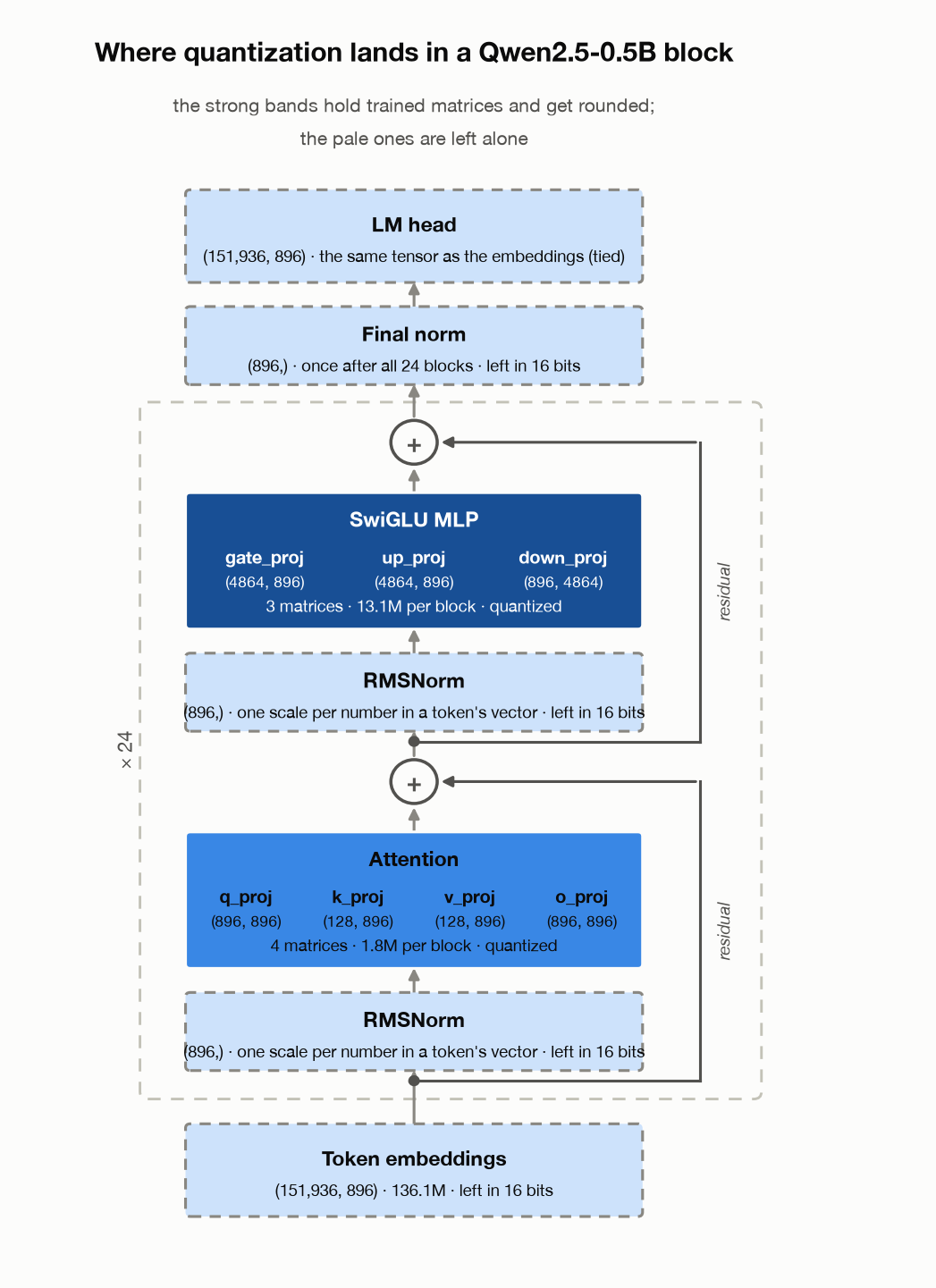
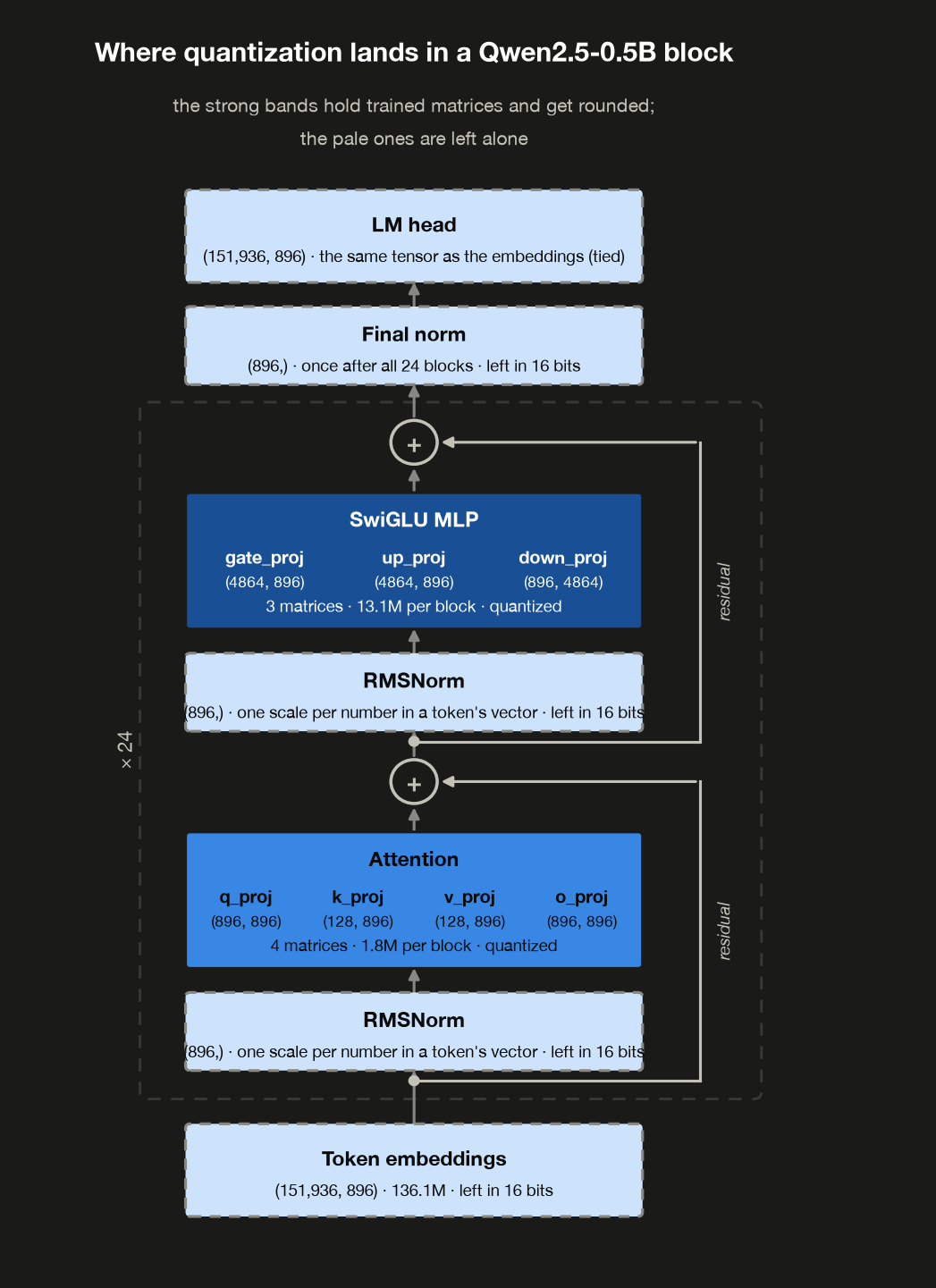
It is post 1’s block diagram with one thing added: the fill now says whether a part gets rounded. The two strong bands hold the seven matrices, each listed with its shape as (out, in). Everything pale is left in 16 bits — the two RMSNorm scales inside each block, one more after all 24, and the embedding table at the bottom, which is the same tensor as the LM head at the top.
The band widths are equal but the shapes inside them are not, and that gap is the thing to carry forward. The MLP’s matrices are 4864 wide where attention’s are 896, which is 13.1M in the MLP against 1.8M in attention, per block. (k_proj and v_proj are narrower still, 128 rather than 896, because grouped-query attention has several query heads share one set of keys and values — post 2’s subject.) Quantization is overwhelmingly something that happens to the MLP. The + nodes and their side rails have no parameters at all, so there is nothing in them to round — and because those rails carry each token’s vector past both halves untouched, rounding the matrices degrades a model gradually rather than breaking it.
what_gets_quantized prints the same inventory as numbers, along with the dimensions every shape in the figure is built from:
1
2
3
4
5
6
7
8
9
10
11
12
13
14
15
16
17
18
19
20
21
  blocks (layers)                    24
  d_model (vector per token)         896
  attention heads / KV heads         14 / 2
  MLP inner width                    4864
  vocabulary                         151,936
  parameters                         494.0M

  'Quantize the model' means the projection matrices and nothing else.
  'tensors' counts stored arrays, not layers: 4 attention matrices in
  each of 24 blocks is 96, and 3 MLP matrices in each is 72.

  part                   tensors  params  share  quantized
  ----------------------------------------------------------
  attention q,k,v,o           96   44.0M   8.9%        yes
  MLP gate,up,down            72  313.8M  63.5%        yes
  embedding (= lm_head)        1  136.1M  27.6%         no
  norms and biases           121    0.1M   0.0%         no

  The MLP carries most of it. Note also that k_proj and v_proj are
  7x smaller than q_proj: this model uses grouped-query attention,
  so several query heads share one set of keys and values (post 2).
d_model is the length of the vector standing for one token as it moves through the stack, and the MLP’s inner width is what gate_proj and up_proj widen it to before down_proj brings it back. Those two numbers, 896 and 4864, are where every shape in the figure comes from.
Three things follow from that table, and they shape the rest of the post. The MLP is where the weights are — its three matrices come to seven times the four attention ones, so quantization is mostly something that happens to the MLP. The norms and biases barely register, 0.1M against 494M, which is why every real tool leaves them in 16 bits without anyone worrying about it. And the embedding table is the one large thing deliberately skipped: over a quarter of the model, untouched, which §6 shows is most of the reason “4-bit” never delivers a 4× saving.
So pick one of the seven to work on: down_proj from layer 11, near the middle of the stack. Nothing distinguishes it — it is an ordinary weight matrix — but it stays the example through §5, so every format below is measured against the same weights and the comparisons are fair.
Now quantize it to INT8. Eight bits gives 256 distinct codes. The scheme below uses 255 of them, spread evenly from $-\text{absmax}$ to $+\text{absmax}$ with one code landing exactly on zero; the 256th is dropped to keep the grid symmetric about zero. Absmax is just the largest magnitude in the tensor, ignoring sign.
That is int8_per_tensor, in full:
1
2
3
def int8_per_tensor(w):
    scale = w.abs().max().clamp(min=1e-12) / 127
    return torch.round(w / scale).clamp(-127, 127) * scale
Three steps, and each line is one of them.
Find the step size. w.abs().max() is the absmax. Dividing it by 127 gives scale, the distance between two neighbouring points on the grid, measured in the weights’ own units. (The .clamp(min=1e-12) only guards the degenerate case of an all-zero tensor, so the next line can never divide by zero.)
Round. w / scale restates every weight as a multiple of that step, so the largest one lands on $\pm 127$ and the rest fall somewhere in between. torch.round snaps each to the nearest whole number, and this is the only place anything is lost — whatever fraction of a step a weight was carrying is gone for good. The .clamp(-127, 127) catches a weight that rounding could nudge one step past the end.
Convert back. * scale returns the numbers to the units they started in.
That last step is worth pausing on, because it says what the function does not do. It hands back an ordinary fp32 tensor, the same size as the one it was given; nothing here saves a single byte. What it produces is the tensor a real 8-bit model would reconstruct when it runs — the weights after a round trip through the grid. That is the right thing to measure, because the question in this section is what the rounding costs in accuracy. The storage saving is a separate calculation, and §6 does it.
The scale, meaning that divisor, is the only design decision in the whole thing, and the rest of this post is about where to put it.
what_rounding_costs calls it on the matrix and prints what the rounding cost:
1
2
3
4
5
6
7
8
9
  One real weight matrix: layer 11 down_proj, (896, 4864), fp32.

  absmax |w|                         0.6133
  std of w                           0.0183
  absmax / std                       33.6

  step = absmax / 127                4.829e-03
  worst rounding error = step/2      2.414e-03
  measured max |q(w) - w|            2.414e-03
The last two lines are the check, and they agree exactly. The error is half a grid step. Nothing more mysterious than that is going on, and the grid step is $\text{absmax}/127$ — set entirely by the single largest weight in the tensor.
Which puts the whole problem in one line: every weight in that matrix is paying for the biggest one. Note the third row — the largest weight is 33.6 standard deviations out. The grid has to stretch that far, while almost all the weights huddle near zero, so most of the 256 levels sit in a region that is essentially empty.
That observation has two possible fixes, and this post measures both. Either narrow what shares a grid (§4), or stop spacing the levels evenly (§5).
2. Where the outliers actually live
So far this post has rounded the model’s weights: the trained matrices from §1, the strong bands in the diagram. Weights sit in the file you downloaded and never change. You can open one up, look at every number in it, choose a grid, round it, save the result, and be finished.
A running model also makes a second set of numbers, and this set never gets saved anywhere. Each token arrives at a layer as a vector, the layer does its work, and a new vector comes out and goes on to the next layer. Those in-between vectors are the activations. They exist only while the model is running, and feeding it different text produces different ones.
You could round the activations too, and there is a real reason to want to. An 8-bit weight multiplied by a 16-bit activation still has to be multiplied in 16 bits, because the weight gets unpacked back to 16 bits before the multiply happens. Rounding the weights alone makes the model smaller and cuts the memory traffic — the win post 2 cared about — but the arithmetic is exactly what it always was. Round both sides and the multiplication itself can be done in whole numbers, which hardware built for it does faster.
Almost nobody ships that. Two reasons.
You would have to choose the grid before you have the numbers. A weight can be studied once, offline, at leisure. An activation does not exist until someone sends a request, and the next request makes different ones — so its grid has to be guessed ahead of time from sample text, or worked out on the spot while a user waits for their answer.
And the numbers turn out to be far worse behaved. That part is measurable, which is what the rest of this section does. §1 showed the damage a grid does is set by the ratio between the largest value on it and a typical one; call that the dynamic range of whatever shares a grid. So the question is a simple one: which set has the wider range — the weights sitting in the file, or the numbers the model makes up as it goes?
First a word for the thing being measured. A model’s numbers are not a flat pile; they are organised into channels — the internal feature dimensions a layer reads and writes.
Which axis that is depends on what you are looking at, and the two tables below make the difference concrete. For a weight matrix, a channel is one row: down_proj.weight has shape (896, 4864), so it has 896 channels, one per output it produces. For the activations — the values flowing between layers, computed fresh for every input rather than fixed at the end of training — a channel is one column: the values arriving at that same down_proj are 4864 wide, so they have 4864 channels, one per input it consumes. Same layer, two different counts, because a matrix has an input side and an output side and each gets its own.
What makes it one idea rather than two is that a channel is always one feature, tracked across everything else. For a weight, across every input it reads. For an activation, across every token in the sequence.
Now, what to measure about them, and why that and not something else.
Start from what §1 established. The grid step is absmax / 127, so the single largest value sharing a grid decides how coarse the grid is for everything on it. Every value then takes the same absolute rounding error, half a step. But the same absolute error means very different things to different numbers: it is a rounding error of a fraction of a percent for a large one and a wrecking ball for a small one. So the number that predicts damage is not how big the largest value is. It is how big the largest value is compared to an ordinary one — because that is how far off the grid’s spacing is for the ordinary values, which is nearly all of them.
Hence a ratio. The median goes on the bottom rather than the mean, because a handful of enormous values drags a mean upward and would hide the very gap being looked for.
And it is measured channel by channel rather than over the whole tensor because of where this is heading. A grid does not have to be shared by every number in a tensor; §4 gives each row one of its own. Measuring per channel is what tells you whether that would help. If the extremes sit in a few channels, splitting the scale isolates them and everyone else goes back to a grid that fits. If every channel is equally wide, splitting buys nothing and the problem is somewhere else.
So: for each channel take its largest magnitude, and express it as a multiple of the median channel’s. A ratio of 1 means a perfectly ordinary channel; 85 means one channel towers over the rest.
The tables report that ratio two ways, because “how bad is the worst one” and “how many are bad” are different questions. max / median is the single worst channel in the tensor. channels > 5x counts how many channels come out above five — a round number standing for “clearly not ordinary”, not a principled threshold. The difference matters: one channel at 85× is a freak you could imagine handling specially, while two hundred channels above 5× is a population you cannot.
where_the_outliers_are measures both. Weights first:
1
2
3
4
5
6
7
  tensor                max / median  channels > 5x  channels
  -------------------------------------------------------------
  L0 down_proj.weight           4.2x              0       896
  L5 down_proj.weight           7.6x              3       896
  L11 down_proj.weight          7.0x              4       896
  L17 down_proj.weight          4.6x              0       896
  L23 down_proj.weight          7.3x              1       896
Tame. No channel is more than about 7× its median neighbour, and at most 4 of 896 exceed 5×. Now the activations. The same function captures the values flowing into those same layers during a real forward pass, using a forward hook, which is PyTorch’s way of asking to be handed a layer’s inputs as they go past, without changing what the model computes:
1
2
3
4
5
6
7
8
9
10
11
12
  tensor         max / median  channels > 5x  channels
  ------------------------------------------------------
  L0 o_proj              7.9x              5       896
  L0 down_proj          11.7x            155      4864
  L5 o_proj              3.8x              0       896
  L5 down_proj          85.5x            224      4864
  L11 o_proj             5.4x              2       896
  L11 down_proj         10.3x             28      4864
  L17 o_proj             5.5x              2       896
  L17 down_proj         20.9x            158      4864
  L23 o_proj             8.2x             22       896
  L23 down_proj         19.1x             97      4864
The down_proj inputs run to 85× their median channel, an order of magnitude worse than any weight tensor. And it is specifically down_proj, the narrowing step at the end of the MLP, which sees the widened vector after the nonlinearity. o_proj, at the end of the attention half, stays in the same mild range the weights do.
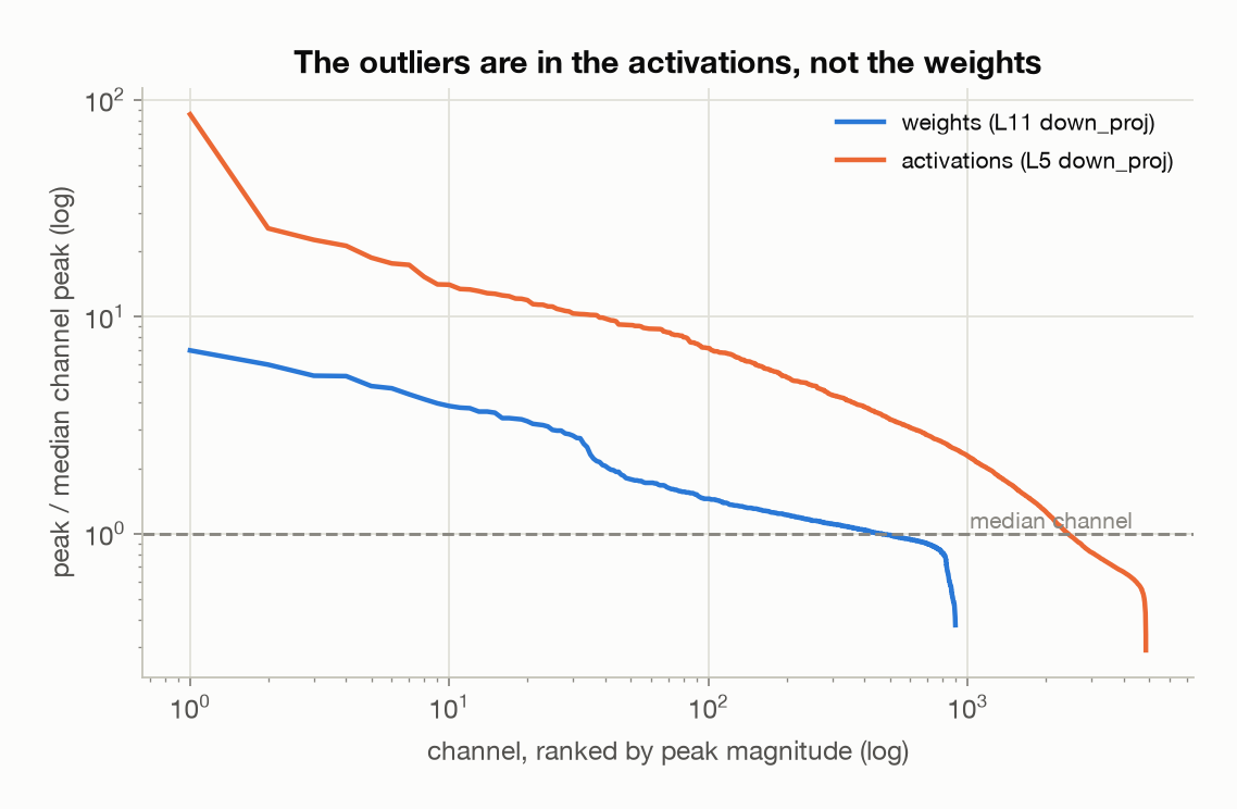
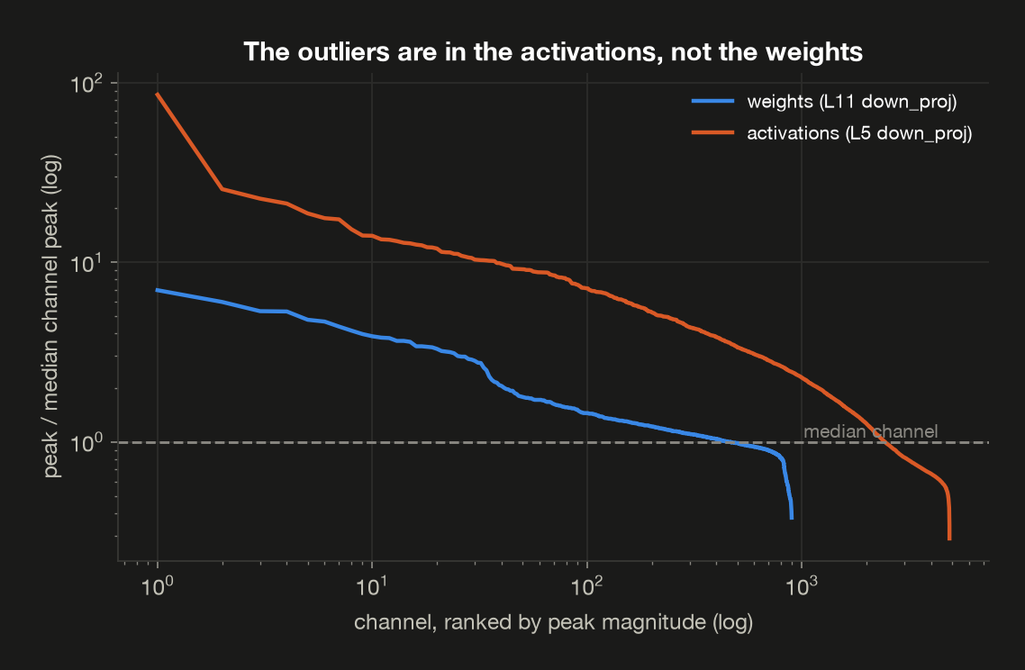
Both axes are logarithmic, and each curve is one tensor’s channels sorted from worst to mildest. The shapes are not far apart — both descend steadily — but the activation curve sits about ten times higher along its whole length, and its first channel juts far above even its own second. That combination is the problem: one extreme channel setting the grid, and behind it a long tail of channels that are also too large to ignore, the 224 counted above. These are the outlier features described in Dettmers et al., LLM.int8() (2022).
Weight-only quantization is what essentially everyone ships (GPTQ, AWQ, bitsandbytes’ NF4), and the reason is the two tables above: weights are well behaved and activations are not. Quantizing activations means confronting an 85× dynamic range on every forward pass; quantizing weights means confronting a 7× one, once, offline.
So do you need to quantize activations?
For most people, no — and not because it is hard, but because it would not buy what you came for.
Go back to what the two options give you. Rounding the weights makes the file smaller and cuts the bytes hauled from memory. Rounding the activations as well lets the multiply run in integer arithmetic. Which of those matters depends entirely on what your hardware is waiting on, and post 2 measured that: generating a token does 0.5 FLOP per byte of weights moved, against 256 for reading a prompt. Generation is not waiting on arithmetic. It is waiting on memory, by a factor of five hundred.
So for generation, weight-only quantization already addresses the actual bottleneck, and quantizing activations on top of it makes the part that was never the constraint faster while adding all the difficulty above. That is the case for almost everyone serving a model.
The exceptions are the workloads that are compute-bound: long prompts, large batches, training. There the 256 FLOP/byte end of that table applies, integer arithmetic is a genuine win, and it is worth the trouble — which is exactly the territory LLM.int8() and SmoothQuant were built for. If you are not in it, quantize the weights and leave the activations alone.
3. Are they the same channels every time?
§2 ends on a tempting thought. If only a couple of hundred channels out of 4,864 are the trouble, why put them on a grid at all? Leave those few in 16 bits, quantize everything else, and the wide range never has to be represented. That is broadly what LLM.int8() does.
The plan has a prerequisite, though: you have to know which channels. If the extreme ones are the same dimensions every time, you can find them once, write the list down, and ship it. If they move around depending on what the model is reading, you would have to find them again on every forward pass — which costs exactly the time quantization was meant to buy.
So the question is whether the outlier channels stay put. The received account says they largely do — Dettmers et al., LLM.int8(): 8-bit Matrix Multiplication for Transformers at Scale (2022), §3.1 — which describes systematic outlier features: specific dimensions that are extreme across inputs and layers alike, in their measurements emerging abruptly once a model passes about 6.7B parameters. That is a checkable claim, so check it.
outlier_persistence takes the worst tensor from §2 — layer 5’s down_proj input, the one at 85× — and runs five unrelated texts through it: English prose, popular science, economics, Python source, and Spanish. For each text it notes which ten channels have the largest magnitudes, then compares those top-ten lists against each other.
Reading the table: each row in the first block takes two of the texts and counts how many channels appear in both of their top-tens, so 3/10 means three in common and seven different. shared by all five inputs intersects all five lists at once. distinct channels across inputs counts how many different channels show up anywhere across the five lists — five lists of ten is fifty slots, so a total near 10 would mean the same channels every time, and near 50 would mean no agreement at all. The final line is a separate experiment: one text, six layers sampled through the stack, their top-tens compared the same way.
1
2
3
4
5
6
7
8
9
10
11
  input pair                  shared of top-10
  ----------------------------------------------
  English prose vs science                3/10
  science vs economics                    2/10
  economics vs Python source              2/10
  Python source vs Spanish                2/10

  shared by all five inputs          2/10
  distinct channels across inputs    41

  shared by all 6 sampled layers     0/10
Not reliably enough to build on. Two channels are in the top ten for all five inputs, including Python source and Spanish, which is not agreement you get by coincidence — there is a real persistent core. But 41 distinct channels turn up across only five texts, so most of the set moves with whatever the model is reading. And across layers there is no overlap at all: knowing layer 5’s outlier channels tells you nothing about layer 11’s.
Be careful about what this does and doesn’t say. The strong systematic version is documented at 6.7B parameters and above — that threshold is LLM.int8()’s own finding, not a rule of thumb — and this is a 0.5B model. Whether the effect sharpens with scale is not measured here — I have no 7B result to offer, and the literature says it would look different. What the measurement does establish is that at this scale you cannot pick the outlier channels once and hard-code them.
So the shortcut is out. You cannot write down a list of dangerous channels once and skip them thereafter, because the list depends on the text and on the layer, and rebuilding it on every forward pass costs the time quantization was supposed to buy.
That is what makes §4’s fix the interesting one: it never has to identify anything. Instead of finding the extreme channels and treating them specially, it stops asking the question — it narrows what shares a grid until an extreme value can only damage its own neighbourhood, whichever value happens to be extreme this time. You do not need to know where the outliers are. You need to stop making everything else share a grid with them.
4. Same bits, different scale placement
Keep the format identical, 8 bits and evenly spaced, and change only the scope of the scale. Per-tensor uses one divisor for everything. Per-channel gives each output row its own — int8_per_channel, next to it in the same file:
1
2
3
def int8_per_channel(w):
    scale = w.abs().amax(dim=-1, keepdim=True).clamp(min=1e-12) / 127
    return torch.round(w / scale).clamp(-127, 127) * scale
One line different, amax(dim=-1, keepdim=True) instead of max(), and it confines each outlier to the row it lives in. A row is the natural unit because a weight matrix is stored as (out_features, in_features): each row holds every weight feeding one output channel, so a row is exactly the group that gets summed together in the matrix multiply. The overhead is one float per row against in_features weights per row, a fraction of a percent.
Error is reported as relative RMSE, which is two lines. Root-mean-square is the ordinary way to average a set of numbers when you want their size and not their sign: square each one, take the mean, take the square root. Do that to the errors, then divide by the same quantity computed on the original tensor, and the answer reads as a percentage of typical magnitude rather than an absolute number whose scale you would have to remember:
1
2
def _rel_rmse(reference, got):
    return ((got - reference).pow(2).mean().sqrt() / reference.pow(2).mean().sqrt()).item()
scale_placement runs that twice on every tensor — once against the per-tensor quantization, once against the per-row one — so the two number columns are the same measurement with the divisor in two different places:
per-tensoris_rel_rmse(w, int8_per_tensor(w)): quantize with one scale for the whole tensor, then ask how far the result moved.per-rowis_rel_rmse(w, int8_per_channel(w)): the same, with one scale per row.ratiois the first divided by the second — how many times less error splitting the scale bought.
A tensor that came back unchanged would score 0%; 100% would mean the error is as large as the values themselves.
Before the numbers, it is worth seeing how lopsided the per-tensor arrangement is. The same function prints what each scale is responsible for:
1
2
3
4
5
6
7
8
  What each scale has to cover, for L11 down_proj:

  weights per scale, per-tensor      4,358,144
  weights per scale, per-row         4,864

  tensor absmax                      0.6133
  row absmax, median                 0.0879
  rows under half the tensor absmax  881 of 896
One divisor for 4.4 million weights, and it is set by the single largest value anywhere among them: 0.6133. But a typical row never gets near that — the median row’s largest weight is 0.0879, about seven times smaller. 881 of the 896 rows never reach even half the tensor’s absmax. So under per-tensor scaling, almost every row in the matrix is being measured on a ruler far too coarse for it, and the 5.4× is what handing each row its own ruler recovers.
1
2
3
4
5
6
  tensor                      per-tensor  per-row  ratio
  --------------------------------------------------------
  L0 down_proj.weight              3.81%    1.14%   3.3x
  L11 down_proj.weight             7.63%    1.41%   5.4x
  L23 down_proj.weight             6.69%    1.14%   5.9x
  L5 down_proj (activations)      58.10%    6.10%   9.5x
Take the weight rows first, because they settle how the rest of this post quantizes anything. Moving the divisor from the whole matrix to each row cuts the error by 3–6× — on layer 11, the running example, from 7.63% to 1.41%. Nothing about the format changed. Still 8 bits, still evenly spaced, still the same 255 levels; the only difference is that an extreme weight now sets the grid for its own row rather than for all 896 of them.
And it is close to free. One extra float per row, against 4,864 weights in that row, works out to 8.007 bits per weight against 8.000 — §5’s table has the figures. Under a tenth of a percent more storage, for five times less damage.
So yes: per-channel is simply the better way to quantize a weight matrix, and there is no interesting case for the alternative. Every serious tool defaults to it, everything after this section uses it, and §5 will show it beating 4-bit NF4 on quality by a wide margin.
Now the last line, which needs a caution before it can be read. The column says per-row, and a row is not the same thing on every line. A weight matrix is (out_features, in_features), so its rows are output channels — for the three weight lines, per-row is per-channel. The activation tensor is (tokens, channels), so its rows are tokens: that last line is one scale per token, not one per channel.
That is not a slip in the experiment, it is the only version anyone could deploy. A per-channel scale for activations would have to be chosen before the activations exist, which is precisely what §3 showed you cannot do. A per-token scale can be worked out from the token itself the moment it arrives, at the cost of one maximum over its 4,864 numbers. That is what LLM.int8() does, and it is why activation quantization is discussed in terms of tokens rather than channels.
For the activation tensor, splitting the scale is the difference between a number you can use and one you can’t. 58% relative error means the quantized tensor barely resembles the original — and the cause is the row from §2: that tensor has a channel 85× its median, and per-tensor scaling makes every other value in the tensor share a grid built to survive it.
But notice where per-token scaling leaves off. It removes the variation between tokens, and that alone is worth 9.5×. What it cannot touch is the variation within a token, across channels — and 6.10% is still four times the error the same format causes on a weight matrix. Getting below that is what SmoothQuant and its relatives are for: they move some of the activation’s range into the weights, where §2 showed there is room to absorb it.
So “is 8 bits enough?” is not a question about 8 bits. The bit width was identical in both columns; what changed was how much dynamic range was forced through a single divisor.
5. NF4: a grid shaped like the data
The other fix attacks the grid instead of the scale. Evenly spaced levels are optimal only if the values are evenly spread, and §1 already showed they aren’t: weights are roughly normal, clustered hard around zero, with an absmax 33 standard deviations out.
NF4, NormalFloat-4 from Dettmers et al.’s QLoRA (2023), puts its 16 levels at the equal-probability quantiles of a standard normal instead. A quantile is a cut point that splits a distribution by share: the 0.9 quantile is the value 90% of the data falls below. Placing levels at equal-probability quantiles means each level claims about the same share of the weights, so none of them is wasted on a region that is nearly empty. The set of levels a format rounds to is its codebook, and NF4’s is derived rather than chosen. nf4_codebook is the derivation, and icdf is what does the work: it is the inverse of the normal distribution’s cumulative function, so handing it a probability returns the value with that much of the distribution below it. Ask for sixteen evenly spaced probabilities and you get back sixteen levels that each cover an equal share:
1
2
3
4
5
6
7
def nf4_codebook():
    dist = Normal(torch.tensor(0.0), torch.tensor(1.0))
    offset = 0.9677083
    positive = dist.icdf(torch.linspace(offset, 0.5, 9)[:-1])
    negative = -dist.icdf(torch.linspace(offset, 0.5, 8)[:-1])
    levels = torch.cat([negative, torch.zeros(1), positive]).sort().values
    return levels / levels.abs().max()
nf4_derivation runs that and compares the result against the table bitsandbytes — the library most 4-bit models are loaded with — actually ships:
1
2
3
4
5
6
  levels derived                     16
  max |derived - bitsandbytes|       5.96e-08

  narrowest step (near zero)         0.0796
  widest step (near +/-1)            0.3038
  ratio                              3.82x
They agree to 6e-08, which is float noise. The table in the library is not a magic set of tuned numbers; it is what falls out of asking where to put 16 levels if the data is normal.
The last three lines are the point. NF4’s levels are 3.82× closer together near zero than at the extremes, which is exactly where the weights are.
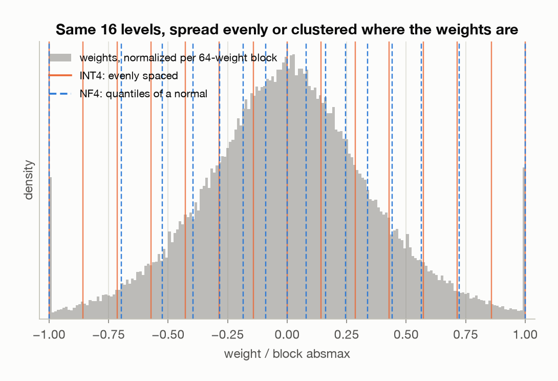
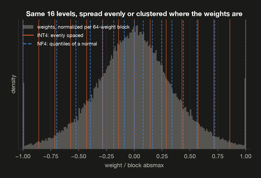
That figure is drawn on block-normalized weights, which is not a cosmetic choice. NF4 is applied blockwise: every 64 weights are divided by their own absmax before meeting the codebook. On a raw axis the 33× ratio from §1 pushes every level of both grids out into empty tails and the comparison shows nothing. Divided by their block’s absmax, the weights form the bell the codebook was designed for, and you can see the dashed NF4 levels crowding the middle where the mass is while the solid uniform levels ignore it. (The spikes at $\pm 1$ are an artifact of the normalization: each block contributes exactly one weight at its own absmax.)
Now measure all of it on the same matrix, at real stored cost. The same function quantizes the matrix five ways and reports error against storage:
1
2
3
4
5
6
7
  format                  rel RMSE  bits/weight incl. scales
  ------------------------------------------------------------
  INT8 per-tensor            7.63%                     8.000
  INT8 per-channel           1.41%                     8.007
  INT4 uniform, block=64    12.21%                     4.500
  NF4 block=64               9.64%                     4.500
  NF4 block=256             11.15%                     4.125
That table is worth reading as a set of controlled comparisons rather than a ranking, because adjacent rows differ in exactly one thing each. Three separate choices are in play — how many levels there are, where those levels sit, and how many weights share a scale — and the table varies them one at a time.
- Rows 1 → 2 change only the scale’s scope. Same 255 levels, same even spacing; the divisor stops covering the whole matrix and covers one row instead. From 7.63% to 1.41%: worth 5.4×, for 0.007 bits per weight.
- Rows 3 → 4 change only where the levels sit. Same 4 bits, same 64 weights per scale, same number of scales. Uniform spacing against normal quantiles, and nothing else. From 12.21% to 9.64%: worth 1.27×, for nothing at all — the codebook is a constant.
- Rows 4 → 5 change only how many weights share a scale. The same NF4 codebook, block 64 against block 256. From 9.64% to 11.15%: 1.16× worse, and it buys back 0.375 bits per weight. That is §4’s trade again, at a finer grain.
- And across the bit widths: per-channel INT8 at 1.41% against NF4 at 9.64% is 6.8× more error for half the storage.
So the three levers are not worth the same, and they are not substitutes for each other. Halving the bit width is the single biggest change to quality here — 16 levels cannot do what 255 can, and no rearrangement of them will fix that. But within a bit width, where you put the scale is the lever that matters and the cheapest one to pull: the same 8 bits span 7.63% to 1.41% depending on nothing but how much of the matrix shares a divisor. Bits set the ceiling; scale placement decides how near it you get.
Which is why NF4 does not beat 8-bit and was never going to. What it does is land within a few points of per-tensor INT8 at half the storage — while per-channel INT8 beats it by a wide margin. Worth holding onto, because “4-bit” gets discussed as though it were strictly better than 8-bit rather than a different point on a curve.
Note the bits column too. NF4 at block=64 carries a 32-bit scale per 64 weights: $4 + 32/64 = 4.5$ bits. A “4-bit” model is a 4.5-bit model. Widening to block=256 brings that to 4.125 and pays for it in error, because more weights then share one absmax — the same trade as §4, at a finer grain.
6. What it actually saves
Quantization is sold in multiples: “4-bit means 4× smaller”. It does not. memory_cost counts what is actually there:
1
2
3
4
5
6
7
8
9
  parameters                         494.0M
  of which embedding (tied)          136.1M  (28%)
  of which other Linear              357.8M  (72%)

  scheme            bits/weight (Linear)  model size  vs fp16
  -------------------------------------------------------------
  fp16 (baseline)                 16.000     942 MiB    1.00x
  INT8 per-channel                 8.036     603 MiB    1.56x
  NF4 block=64                     4.500     452 MiB    2.09x
The embedding table in that first block is worth explaining, because it turns out to be the single biggest reason the saving disappoints. A model cannot do arithmetic on text, so before anything else happens each token is looked up in a table that hands back a vector of numbers standing for it. The table has one row per token the model knows — its vocabulary — which for this model is about 150,000 rows, and that is a fixed cost regardless of how deep the model is.
Nominally 16 → 4 bits is a 4× cut. Measured, it is 2.09×. Two things dilute it, and both are counted rather than estimated:
- The scales ride along. 4 bits become 4.5, an eighth of the saving gone before anything else.
- 28% of this model is an embedding table that nobody quantizes, and it stays at 16 bits. Small models are hit hardest here — the embedding is a fixed cost set by vocabulary size, so it is a much larger share of a 0.5B model than of a 70B one. Expect the ratio to look better at scale, though this post doesn’t measure that.
These are analytic figures — parameter counts times bits per weight, not a measurement of a file on disk. They’ll track a real checkpoint closely but won’t match it to the byte, since formats carry headers and padding of their own.
7. Perplexity says fine; the tail says otherwise
Now the question that matters: does the model still work?
The standard answer is perplexity, and it is worth building up rather than quoting, because its blind spot follows directly from how it is made.
Run some real text through the model. At each position the model has produced a probability for every token in its vocabulary, and one of those tokens is the one that actually came next. Pull out the probability it gave that correct token. A confident, well-fitted model gives it a high probability; a damaged one gives it a lower one.
Now turn that into a score. Take the logarithm of each of those probabilities and negate it, so a probability of 1 scores 0 and anything less scores positive — that is how much the model was surprised at that position. Average the surprise over every position. Then exponentiate the average, which converts it out of log units back into a count. That count is perplexity, and it reads as: the model was as uncertain as if it had been choosing uniformly among this many options at each step. A perplexity of 20 means roughly a 20-way guess, and lower is better.
That is four lines of quality, and the third one is where the rest of this section comes from:
1
2
3
4
def perplexity(lg):
    logp = torch.log_softmax(lg[:, :-1], dim=-1)
    nll = -logp.gather(-1, ids[:, 1:].unsqueeze(-1)).squeeze(-1)
    return nll.mean().exp().item()
nll.mean() is an average over every token in the passage. Every conclusion in this section falls out of that one call: an average is a single number standing in for thousands, and it has no way to report that a few of them are far from the rest.
Evaluating perplexity needs text, so the demo ships a fixed 550-token passage covering six unrelated topics. That choice is load-bearing, and my first attempt got it wrong: it repeated one paragraph a dozen times, which is far easier to predict, and it reported NF4 costing 2.5% where honest non-repeating prose reports 15.5%. Repetitive eval text flatters a quantized model.
So alongside perplexity, measure something an average cannot see. Perplexity looked at one number per position, the probability of the token that actually came next. But the model produced a probability for every token in its vocabulary at that position, and quantizing shifts the whole shape of that distribution. KL divergence puts a single number on how far the shape moved: zero means the two distributions are identical, larger means the model now expects something different. It is reported per token, in nats — the unit you get when the logarithms are natural ones, as they were above. Here 0.18 nats is a small but real change of mind and 10 nats is a different model.
quality runs each scheme against the unquantized reference and reports both:
1
2
3
4
5
6
  scheme                perplexity  vs fp32   mean KL    max KL  max/mean
  -------------------------------------------------------------------------
  fp32 reference            20.869        —         —         —         —
  INT8 per-channel          20.913   +0.21%  2.60e-03  1.76e-01       68x
  NF4 block=64              24.104  +15.50%  1.57e-01  1.09e+01       69x
  NF4 block=64, + head      26.486  +26.92%  2.44e-01  1.09e+01       45x
Before anything else, which scheme is better? On quality it is not close: INT8 per-channel, by every column. Perplexity +0.21% against +15.50%, and mean KL 2.60e-03 against 1.57e-01, sixty times smaller. Worth noting that the gap is wider here than it was on the weights themselves — §5 measured per-channel INT8 at 6.8× less weight error than NF4, and by the time that reaches the model’s predictions it is 60×. Small differences in the weights do not stay small after 24 layers.
What the table deliberately does not show is the other half of the trade. NF4 is half the size (§6 has the storage figures) and that is the entire reason anyone reaches for it. So the honest reading is: 8-bit per-channel if quality is what you are optimising, 4-bit if the model has to fit somewhere it otherwise wouldn’t, and the numbers above are what the second choice costs.
Read the INT8 row twice. Perplexity moved 0.21%. That would clear any ship/no-ship threshold anyone sets — you would call it lossless and move on. In the very same run, one token’s predicted distribution moved 68× the average.
Both numbers are correct. Perplexity is a mean over hundreds of tokens, and a mean is precisely the statistic that cannot see a tail. The same function sorts every token’s KL and reports where the damage sits, using the quantiles from §5 — quantile 0.99 being the level only the worst 1% of tokens exceed:
1
2
3
4
5
  INT8 KL at quantile 0.5            1.730e-03
  INT8 KL at quantile 0.9            4.341e-03
  INT8 KL at quantile 0.99           1.194e-02
  INT8 KL at quantile 0.999          9.441e-02
  INT8 KL at quantile 1.0            1.756e-01
Flat across the bulk, then a hundred-fold climb in the last tenth of a percent.
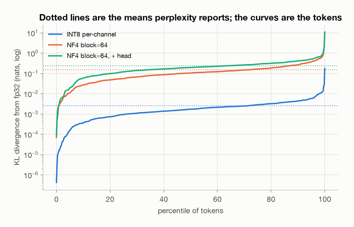
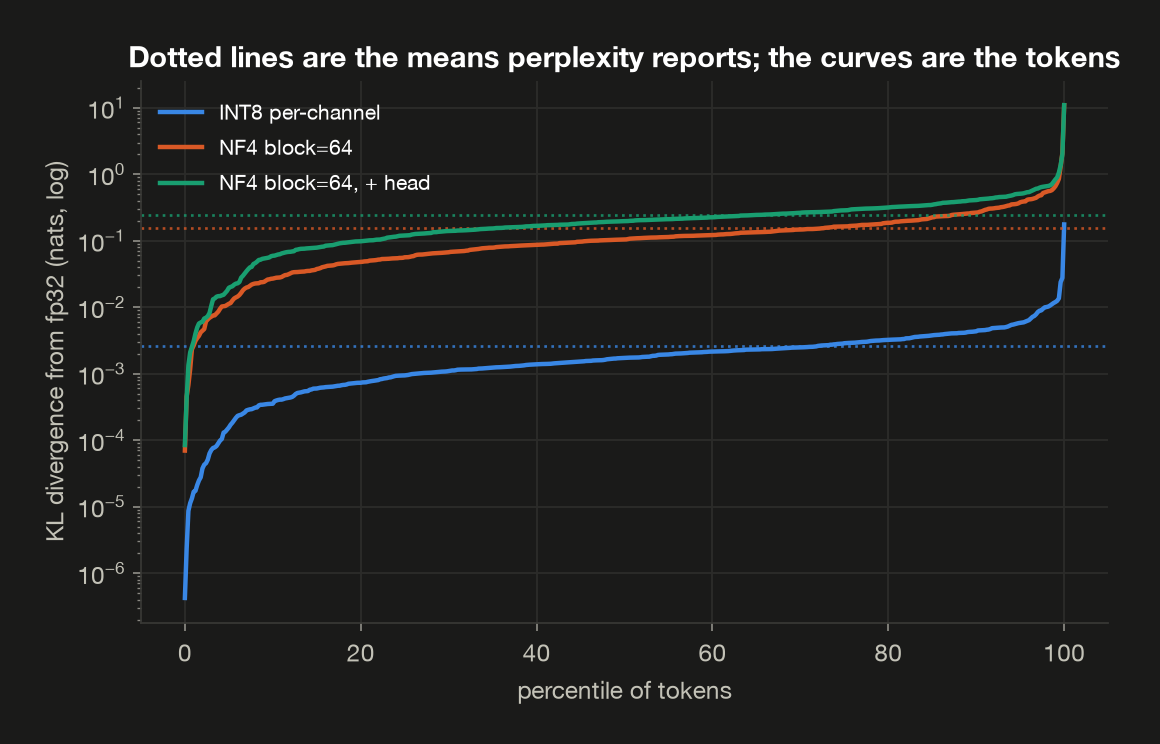
Each dotted line is the mean — the kind of number a perplexity comparison reports. Each curve is where the tokens actually are. The means sit above the median of their own curves, dragged up by a handful of tokens at the right edge, and every curve hooks sharply upward in its last few percent. The tokens that changed most are exactly the ones a mean is worst at reporting.
Whether that matters depends on what the changed tokens are. Perplexity treats every position as interchangeable; a product does not. A model that is imperceptibly worse on ordinary prose and meaningfully worse on the rare tokens carrying names, digits, code syntax, or a refusal has a problem that perplexity is not built to report, and this post doesn’t identify which tokens moved — only that some did, by a lot. That is the honest boundary of the measurement, and it is also the argument for evaluating on what you actually care about.
The line that costs more than the format
The bottom row is a different lesson. In Qwen2.5-0.5B the embeddings are tied: lm_head.weight and embed_tokens.weight are the same tensor under two names, sharing storage.
A tensor is one array of numbers, and two names can point at the same one. data_ptr() returns the address where a tensor’s numbers actually live, so comparing the two addresses settles whether they are one tensor or two copies. memory_cost runs that check:
1
  lm_head.weight is embed_tokens.weight  yes
So the natural-looking loop, “quantize every nn.Linear” — every one of the model’s matrix-multiply layers — also quantizes the embedding table, which every token in the sequence reads on the way in. Perplexity goes from +15.50% to +26.92%: that single decision costs 11 points, comparable to the entire gap between 8-bit and 4-bit. Real tools exclude the head and embeddings by default, and this is why.
8. What follows from all this
| If you’re deciding | The thing that decides it |
|---|---|
| 8-bit or 4-bit? | Not error alone — per-channel INT8 was 1.41% against NF4’s 9.64%. 4-bit is a memory decision you pay for in quality, not a free upgrade. |
| Weights only, or activations too? | Weights only, for generation. Decode does 0.5 FLOP per byte of weights moved, so it waits on memory, and weight-only already fixes that. Activation quantization speeds up arithmetic you were not waiting on — worth it only for compute-bound work like long prompts, big batches or training. |
| Per-tensor or per-channel? | Per-channel, always. It costs one float per row and was worth 3–6× on weights, 9.5× on activations. |
| Is my quantized model safe to ship? | Not answerable by perplexity. It moved 0.21% while the worst token moved 68× the mean. Look at the tail, and at the tokens you actually care about. |
| Why is my 4-bit model only half the size? | Scales (4 → 4.5 bits) and the embedding table you correctly left alone (28% here). |
| Why did quality collapse when I quantized everything? | Check whether your embeddings are tied. lm_head is often the same tensor as embed_tokens. |
Underneath all of it, quantization damage is a dynamic-range problem rather than a bit-width problem. Every result here reduces to who was forced to share a divisor with whom — per-tensor against per-channel, block 64 against block 256, activations against weights. Bits set the ceiling on how good it can get; scale placement decides how much of that ceiling you reach.
9. Sidebar: the probe
One question to close on — the kind this material gets asked, and what separates an answer that sounds right from one that is.
“You quantized the model to 4-bit and perplexity barely moved. Is it safe to ship?”
The tempting answer: “Yes. Perplexity is within a percent of the original, so it’s effectively lossless.”
That is the answer the number invites, and it treats an average as a guarantee.
A better answer comes in three moves.
1. Flat perplexity is necessary, not sufficient. It is a mean over every token in the test passage, and a mean has no way to report that a few of its terms sit nowhere near the rest.
2. So the real question is which tokens moved. Measured token by token, INT8 weight-only moved perplexity 0.2% while the worst single token’s predicted distribution moved 68× the average — flat across the bulk, then a hundred-fold climb in the last tenth of a percent. If that damage lands on the rare tokens carrying names, numbers or code syntax, perplexity will never show it and your users will.
3. And check what actually got quantized. If the embeddings are tied to lm_head, a loop over “every linear layer” hits the embedding table as well — which cost 11 points of perplexity here, more than the entire gap between 8-bit and 4-bit.
What the question is really testing is whether perplexity is being treated as a summary statistic with known blind spots, or as a verdict.
What’s next
Post 5 is mixture-of-experts — the other way to make a large model cheap to run, and one that trades in a completely different currency. Quantization shrinks every weight; MoE keeps them all and simply declines to use most of them on any given token. The interesting questions there are what the router actually learns, why “active parameters” is the number that predicts speed while total parameters predicts your memory bill, and what happens to a batch when every sequence in it wants a different expert.
Appendix: all notation
Every symbol this post uses, in one place. Post 1’s appendix covers attention’s own notation, and post 2’s the memory and serving terms.
| Symbol | Means | In this post’s runs |
|---|---|---|
| $w$ | a weight tensor, before quantization | e.g. $(896, 4864)$ |
| $q(w)$ | the same tensor after rounding to the format’s levels | same shape, fewer distinct values |
| $s$ | the scale: the divisor applied before rounding | one per tensor, row, or block |
| absmax | the largest magnitude in whatever shares a scale | 0.6133 for L11 down_proj |
| step | spacing between adjacent levels, $\text{absmax}/127$ for INT8 | 4.829e-03 |
| $b$ | bits per stored weight, scales included | 8.007, 4.5, 4.125 |
| block | how many weights share one scale, in a blockwise format | 64 or 256 |
| channel | one row of a weight matrix, or one feature dimension of an activation | 896 or 4864 of them |
| max/median | a channel’s peak magnitude over the median channel’s — the outlier measure | 4–7× weights, 10–85× activations |
| rel RMSE | root-mean-square error over the original’s root-mean-square | 1.41% to 58.10% |
| PPL | perplexity — how surprised the model is by held-out text, lower being better | 20.869 unquantized |
| $D_{KL}$ | KL divergence in nats between two predicted distributions, per token | mean 2.6e-03, max 1.76e-01 |
| INT8 / INT4 | integer formats with evenly spaced levels, symmetric about zero | 255 levels ($\pm 127$) and 15 ($\pm 7$) |
| NF4 | NormalFloat-4: 16 levels at the quantiles of a normal | derived, matches bitsandbytes to 6e-08 |
| fp32 / fp16 | 32- and 16-bit floating point — four and two bytes a number | fp32 reference, fp16 baseline |
Three things worth keeping straight:
- Per-tensor, per-channel, and blockwise are the same idea at three grains. Each names how many weights share one scale: all of them, one row’s worth, or 64. Every quality result in this post is a consequence of that number, not of the bit width beside it.
- “4-bit” is a level count, not a storage cost. 16 levels is what makes it 4-bit; the fp32 scale per block is what makes it 4.5 bits on disk. Both numbers are honest and they describe different things.
- Error and divergence answer different questions. Relative RMSE (§4, §5) measures how far the weights moved and is a property of the format alone. KL divergence (§7) measures how far the predictions moved and is a property of the whole model. A format can look bad on the first and fine on the second, which is roughly what INT8 does.
References
- Dettmers et al., LLM.int8(): 8-bit Matrix Multiplication for Transformers at Scale (2022) — where §2’s outlier features are described, and the mixed-precision decomposition that works around them.
- Dettmers et al., QLoRA: Efficient Finetuning of Quantized LLMs (2023) — NF4, its derivation from the normal distribution, and blockwise scaling. §5.
- Frantar et al., GPTQ: Accurate Post-Training Quantization for Generative Pre-trained Transformers (2022) — weight-only quantization that uses second-order information rather than absmax alone.
- Lin et al., AWQ: Activation-aware Weight Quantization for LLM Compression and Acceleration (2023) — uses the activation outliers of §2 to decide which weights matter, rather than treating all of them alike.
- Xiao et al., SmoothQuant: Accurate and Efficient Post-Training Quantization for Large Language Models (2022) — the other response to §2: migrate the activation range into the weights, where it is survivable.
- Code for this post:
llm-architectures-refresher,uv run demo04.