LLM Architecture Refresh [5]: Mixture-of-Experts, and Why Sparsity Doesn't Survive a Batch
Taking a real 64-expert model apart to find out what the router learns, why active parameters predict speed while total parameters predict your memory bill, and where per-token sparsity quietly disappears.
A model that mostly declines to run
Post 1 took a transformer block apart and put a cost on every piece. One finding matters more here than anything else: the feed-forward network holds more of a model’s parameters than attention does.
The feed-forward network, or FFN, is the per-token stack of matrix multiplies that sits after attention in every transformer block. Attention is where tokens look at one another; the FFN is where each token is transformed on its own. You will also see it called the MLP, short for multi-layer perceptron, which is what most model code names it, including the code for OLMoE, the model measured in this post. I will call it the FFN.
The three posts since then each attacked one of three costs of running a trained model: how much arithmetic it does, how much memory it occupies, and how many bytes it has to move through the hardware while doing that arithmetic.
Post 2 removed work that was being repeated. Instead of recomputing keys and values at every generation step, it stores them in a KV cache. For a 64-token prompt followed by 512 generated tokens, running without the cache pushes 284× as many tokens through the model: 163,584 against 576. The price is memory: for a 128k-token conversation in Llama 3.1 8B’s shape, keeping the cache holds up to 2.0× more memory than recomputing would, and holds it for the whole conversation. Both numbers are worked through step by step in the appendix.
Post 3 removed work that was being written down only to be fetched back. FlashAttention computes attention one tile at a time, so the GPU moves 3.9× fewer bytes between its large main memory and the small, fast memory close to its arithmetic units.
Post 4 stopped being exact on purpose. By storing each weight in fewer bits, it cut the memory the weights take by 2.09×, from 942 MiB to 452 MiB (a MiB, or mebibyte, is $2^{20}$ = 1,048,576 bytes).
They also differed in what they did to the model’s output. The KV cache leaves the computation unchanged: generating with or without it produces the same tokens. FlashAttention computes the same function mathematically, but changes the order of floating-point operations, which introduces tiny differences in the last few bits: about 1e-6 on post 3’s test, against 0.6 for sliding-window attention, which really does approximate. Quantization is different: it deliberately changes the computation by representing weights with fewer bits.
All three techniques operate on a model you already have. Mixture-of-experts makes a different move: it changes the model you build. Instead of sending every token through the same large FFN, an MoE model builds many smaller FFNs, called experts, and sends each token through only a few of them.
That shifts the three costs unevenly. Per token, the arithmetic falls to a fraction. Memory doesn’t fall at all. The bytes a token moves fall as well, but only while it is processed on its own, which §6 shows doesn’t last.
Think of it as a firm with a hundred specialists on staff. A question about a contract doesn’t go to all hundred people. A partner reads it, decides which specialists would be useful, and sends it to three of them, and only those three bill hours to that question. The other ninety-seven haven’t gone anywhere, though. They are still on the payroll, and the firm still pays for desks for all hundred.
So the firm pays two different bills, and only one of them got smaller. The hours billed depend on how many specialists you use; the rent depends on how many you employ. That is the central trade of mixture-of-experts. The hours are compute and the desks are memory: for each token the model multiplies through only a handful of experts, but every expert’s parameters still have to live somewhere, ready in case a later token is routed to it. §5 puts measured numbers on both bills.
The analogy holds only up to a point. Nothing guarantees that neural-network experts divide their work into anything like tax, litigation or employment law; “expert” is the name the component was given, not a promise about what it learns. §4 looks at what the router learns to do.
The model measured in this post has 64 experts in each layer and activates 8 of them per token. Those two numbers are design choices rather than part of the definition, and §1 looks at where they come from.
Nothing is approximated here. OLMoE was trained with this routing from its first step, so the model you run is the model that was trained, and a small learned component, the router, decides which experts each token gets.
The arithmetic is strange the first time you see it. The model in this post has 6.9 billion parameters, and for any one token it activates about 1.2 billion of them. The other 5.7 billion sit in memory, untouched by that token, waiting for other tokens that need them. That is the sense in which this is a model that mostly declines to run.
The whole architecture is on one page below, and every number on it is measured later in the post. Panel 1 is the whole model and panel 2 opens up one MoE layer. The grid of numbered boxes in panel 2 is that layer’s 64 experts, one box per FFN, and the eight filled boxes are the experts selected for one real token.
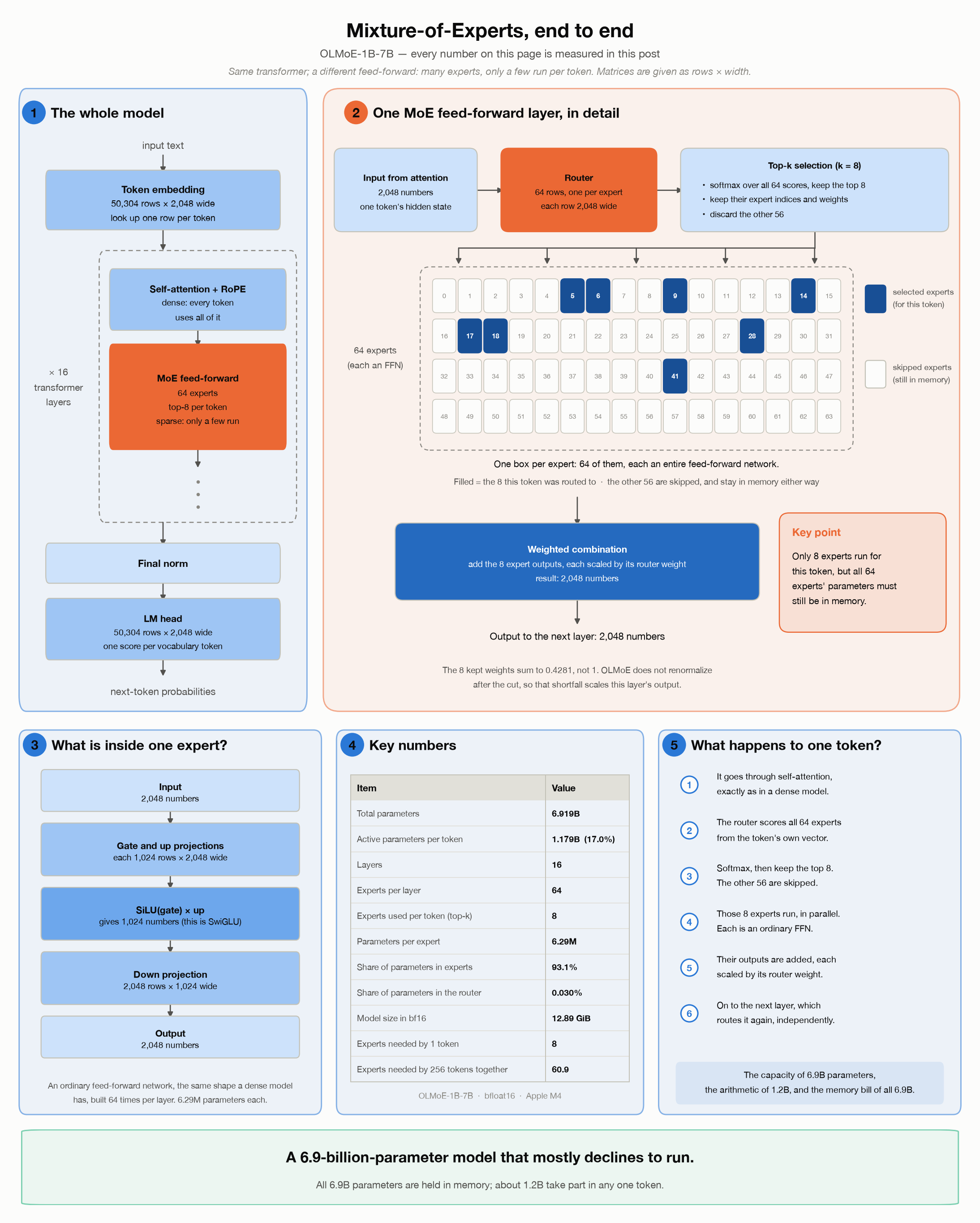
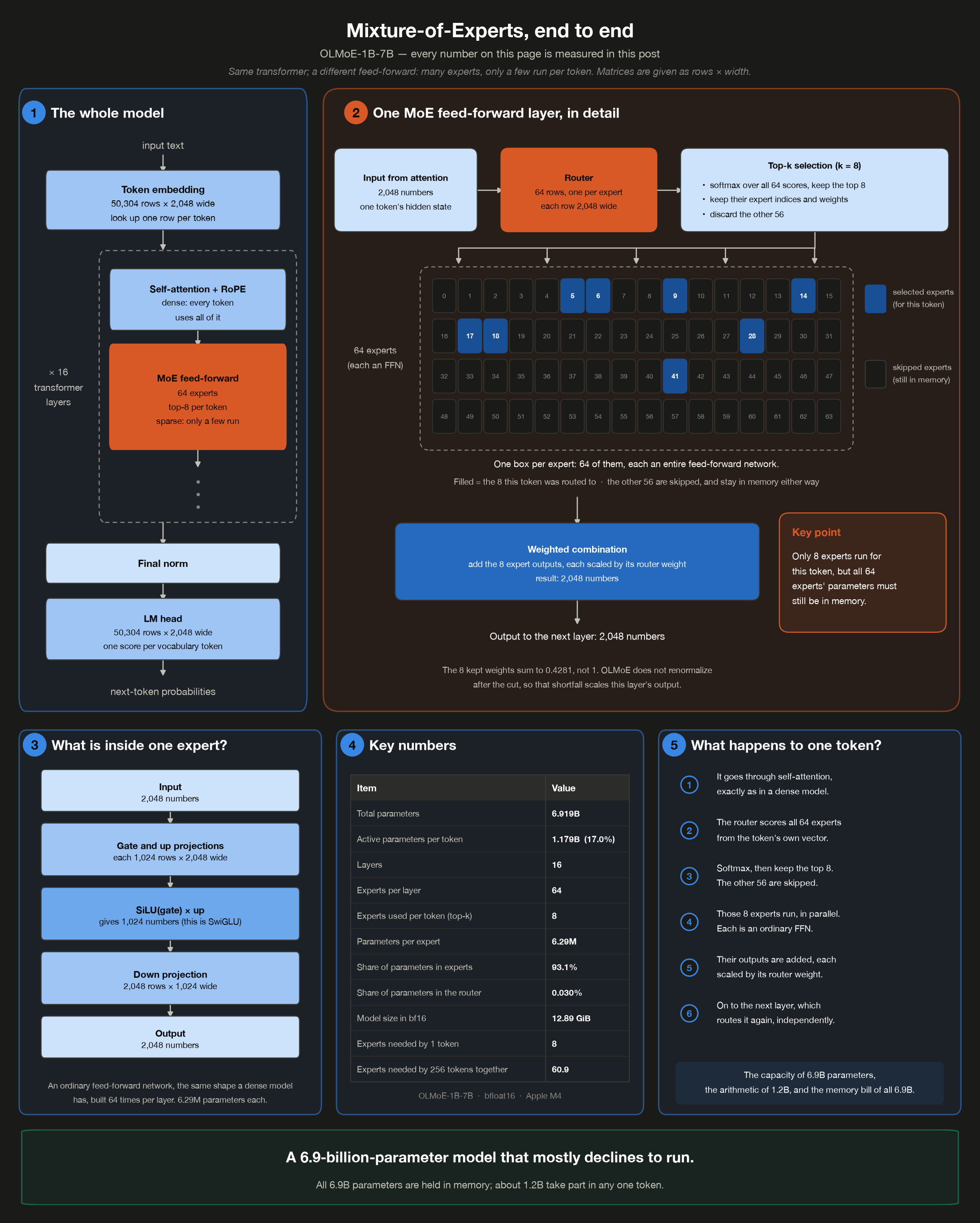
The rest of this post is about how the model decides which eight to wake up, and what letting the other fifty-six sleep actually buys, and costs.
Setup
Everything below is measured, and you can re-run all of it:
1
2
3
git clone https://github.com/bearbearyu1223/llm-architectures-refresher
cd llm-architectures-refresher
uv sync && uv run demo05
The code is in demos/d05_moe.py. Every number this post measures is printed by that program, and each block of its output, which I call a receipt, names the function that printed it. Numbers taken from other models’ configurations or papers link to their source instead.
The model is OLMoE-1B-7B from the Allen Institute for AI (Ai2): the paper, the weights, and the training code and data.
Its name carries the central idea of this post. OLMo is Ai2’s family of fully open language models (Open Language Model), the E stands for experts, and 1B-7B means that about 1 billion parameters are active for each token even though the model holds about 7 billion in total. The full checkpoint name adds 0924, for its September 2024 release.
Both numbers are rounded, and §1 measures them exactly: 6.92B parameters exist, and 1.18B of them are active for a token, or 1.28B if you also count the embedding table the token is looked up in.
Why this model?
The choice wasn’t casual. Like post 4, this post needs a trained checkpoint. A router with random weights has learned nothing about where to send tokens, so the routing behaviour §4 examines only exists after training; the architecture alone doesn’t produce it.
OLMoE suits the experiment for two reasons. The first is that it’s fully open: its weights, training data, code and training logs are all published (Muennighoff et al.), along with intermediate checkpoints saved partway through training. That makes it possible to study how its routing developed and not only where it ended up, although this post measures only the finished model.
The second is that it’s a clean version of the mechanism. Each layer has 64 experts and sends each token to 8 of them, with neither of the two common variations. There is no shared expert, an extra FFN that every token passes through regardless of routing, and the model wasn’t upcycled, which means built by copying a trained dense model’s FFN into many experts and continuing training from there. OLMoE was trained sparse from scratch. That turns out to matter for what its router learned in §4, and §9 comes back to why.
Why bfloat16?
It also has to fit on the laptop running these experiments, which leads to one deliberate break from post 4: this demo loads the model in bfloat16 (bf16), which stores each number in 2 bytes, rather than fp32, which uses 4. At 6.92B parameters the weights alone come to 25.8 GiB in fp32 (a GiB is $2^{30}$ = 1,073,741,824 bytes), more than this laptop’s 24 GiB of memory, and to 12.9 GiB in bf16, which fits.
This is less of a compromise than it sounds, because bf16 is the precision OLMoE was released in. Its published configuration lists bfloat16, so the demo runs the model as its authors ship it rather than a reduced copy. The two kinds of number in this post are affected differently, though. Parameter counts, and everything derived from them, don’t depend on precision at all. Routing measurements, such as which experts a token picks and with what weights, come from a forward pass run in bf16, so an fp32 run could move their last digits. The fp32 model doesn’t fit on this machine, so a full comparison isn’t made here, though §2 checks the router step itself and finds its choices unchanged.
Table of Contents
Skip to the short version for the findings without the derivations.
- Where the parameters are
- The router, which is smaller than you would guess
- One token, routed
- What the router learns
- Two bills: memory and time
- Sparsity does not survive a batch
- When the model spans many GPUs
- Nothing balances the load for free
- How an MoE is trained, and where “mid-training” fits
- What follows from all this
- Sidebar: the probe
Plus three appendices at the end: counting every parameter, which derives §1’s census tensor by tensor; all notation, if a symbol ever goes by without introduction; and where the KV cache numbers come from, for the two numbers the opening section borrows from post 2.
The short version
A mixture-of-experts layer replaces one FFN with many smaller ones, called experts, plus a small router that picks a few experts per token. “Sparse” here means only the picked ones run.
- The experts are essentially the model. 93.1% of OLMoE’s parameters are experts, against 3.9% for attention. A token activates 17.0% of the total (§1).
- The router costs almost nothing. One matrix per layer, 64 rows each 2,048 wide, 2.10M parameters, 0.030% of the model, deciding how the other 93% get spent (§2).
- Routing is a softmax, a cut, and a weighted sum (softmax turns raw scores into probabilities that add to 1), and OLMoE doesn’t renormalize after the cut. The eight kept weights on the token walked through in §3 sum to 0.4281, not 1, so the router’s confidence becomes a scale on the layer’s output.
- The router does specialize, and it can be measured. Two halves of the same passage route differently by 0.216; the three pairs of different text average 0.554, 2.56× that noise floor, and the gap widens with depth (§4).
- Active parameters predict time; total parameters predict memory. Forcing all 64 experts on costs 2.12× the elapsed time and zero extra bytes of weights (§5).
- Per-token sparsity is not batch sparsity. One token needs 8 experts of 64. Two hundred and fifty-six tokens together need 60.9, and 63.7 if the batch mixes domains the way a real one does (§6). That is why an MoE saves arithmetic without saving memory.
- Splitting the experts across GPUs makes the router a network problem. With 64 experts on 8 GPUs, one token’s eight experts land on 5.54 different GPUs on average (§7).
- Nothing keeps the experts equally busy on its own. The busiest expert in layer 0 takes 5.71× an even share, and four experts in the last layer go unused by the test passage (§8).
- Training updates every router row but only the chosen experts. For one token, all 64 router rows get a gradient through the softmax, and only the 8 chosen experts do; a hand-derived formula matches autograd to 1.5e-8 (§9).
- MoE is an architecture, not a training stage. The router and the experts learn together during pre-training, and the same model then carries on through mid-training and post-training unchanged (§9).
1. Where the parameters are
Start with the question post 4 opened on, because for an MoE it has a much more interesting answer: which parts of the model does this technique even touch?
For quantization the answer was “nearly all of it, a bit at a time.” For mixture-of-experts the answer is that it touches one component, the FFN, and replaces it with sixty-four smaller ones.
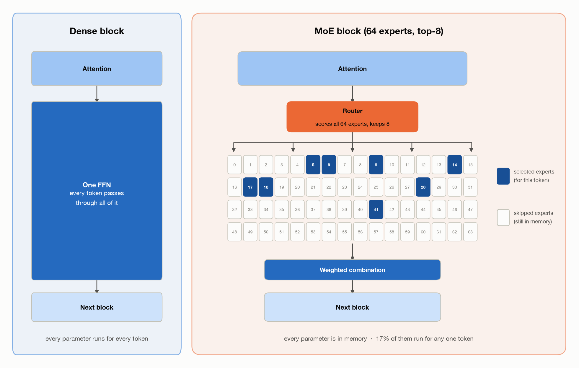
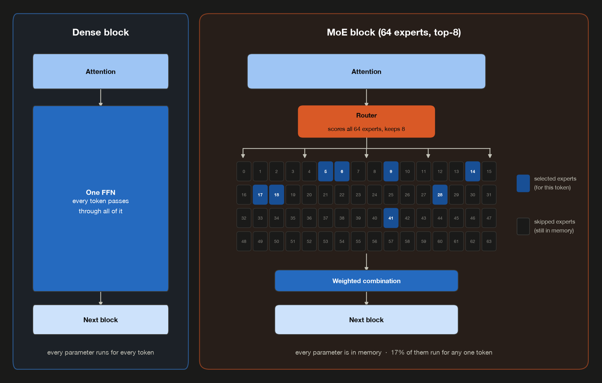
The two columns line up row for row, so the only difference is the feed-forward part: attention and the next block are unchanged, and the single FFN becomes a router, 64 experts and a weighted combination. The eight filled boxes are the experts this post’s own demo routed the word ' harbour' to in layer 0, so the picture and §3’s table are the same measurement.
Counting the parameters by role (where_the_parameters_are):
1
2
3
4
5
6
7
8
9
10
11
12
13
14
15
  role          parameters   share
  ----------------------------------
  experts           6.442B   93.1%
  attention         0.269B    3.9%
  embed + head      0.206B    3.0%
  router             2.10M  0.030%
  norms              0.07M  0.001%
  TOTAL             6.919B  100.0%

  experts per layer                  64
  experts used per token             8
  parameters in one expert           6.29M
  total parameters                   6.919B
  active parameters per token        1.179B
  active share                       17.0%
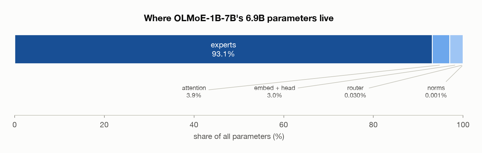
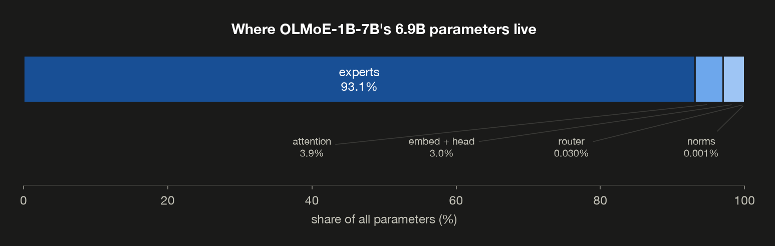
Every number in that table is a parameter count: how many learned numbers the model stores. Each one comes from multiplying out the shapes of the model’s weights, since a matrix of $R$ rows, each $W$ numbers wide, holds $R \times W$ parameters. Appendix: counting every parameter does that for every tensor in the checkpoint, from the query projection to the final norm, and checks the total against the checkpoint’s own count. The number that matters here comes straight out of it: one expert holds 6,291,456 parameters, and 64 experts in each of 16 layers make 6,442,450,944 of them, the 93.1%.
A token doesn’t use all of them. Its active parameters are the ones its arithmetic uses (what_one_token_uses):
1
2
3
4
5
6
7
8
9
10
11
  part                             parameters
  ---------------------------------------------
  8 of 64 experts, x 16 layers    805,306,368
  attention, all of it            268,500,992
  router, scores all experts        2,097,152
  norms                                67,584
  LM head, a full multiply        103,022,592
  embedding table, a lookup       not counted
  active total                  1,178,994,688
  active share of total              17.04%
  active if the lookup is counted    1.28B
Attention, the router and the norms run in full for every token. Of the experts, only 8 of 64 run in each layer, so the expert term is $8 \times 6{,}291{,}456 \times 16$. The LM head is a full matrix multiply, so it counts. The embedding table doesn’t, because a token enters it by lookup: the model reads out one row by position, which multiplies nothing. Counting it anyway gives 1.28B. Either way, the result is the 17.0% that the design exists to produce.
Why sixty-four?
Nothing so far explains where 64 and 8 came from. They’re neither arbitrary nor universal: they’re OLMoE’s choices, set in its configuration. Other models choose differently. Mixtral 8x7B has 8 experts per layer and picks 2 (config). Qwen3-30B-A3B has 128 and picks 8 (the Qwen3 Technical Report’s Table 2, and its config). DeepSeek-V3 has 256 routed experts plus one shared expert, and picks 8 of the 256 (the DeepSeek-V3 report’s §4.2, and its config). The mechanism is the same in all of them; the two numbers are a design decision made per model.
The useful way to read them is that they aren’t two independent knobs. Call the number of experts each token is routed to $k$; for OLMoE, $k = 8$. What a token costs is $k$ multiplied by the width of one expert, and that product is the real budget (why_this_many_experts):
1
2
3
4
5
6
7
8
  model width (hidden_size)          2048
  one expert's width                 1024
    as a multiple of the model width 0.50x
  width actually used per token (8 x 1024) 8192
    as a multiple of the model width 4.00x
  width held in total (64 x 1024)    65536
    as a multiple of the model width 32.00x
  capacity over compute              8x
An ordinary dense FFN is conventionally about 4× the model width, and the dense sibling from the same lab, OLMo-2-1B, has exactly that: hidden 2,048, FFN width 8,192. OLMoE’s eight chosen experts come to 8 × 1024 = 8192, which is the same number. Per token it does precisely as much feed-forward arithmetic as the dense model of its shape. What it adds is the other 56 experts, which is why it holds 8× the FFN capacity for the same per-token cost.
So the number of experts per token, $k$, is set by the compute you’re willing to spend, and the total number of experts is set by the capacity you want. That leaves one genuine question: given a fixed budget on both, do you want a few wide experts or many narrow ones? Holding both budgets fixed and varying only how finely they’re cut (why_this_many_experts):
1
2
3
4
5
6
  experts  each of width  used per token  possible combinations
  ---------------------------------------------------------------
  8                 8192               1                      8
  16                4096               2                    120
  32                2048               4                 35,960
  64                1024               8          4,426,165,368
Every row in that table stores the same number of parameters and runs the same arithmetic per token. What changes is how many distinct combinations of experts a token can be assigned to: 8 at the coarse end, 4.4 billion at the fine end. A model with 8 experts picking 1 has eight possible behaviours at that layer. OLMoE has more than four billion.
That’s the argument for fine-grained experts, and it’s the reason each of OLMoE’s experts is half the model width rather than four times it. It isn’t free: more, smaller experts mean more routing decisions, more scattered memory access, and a token with more experts to reach touches more GPUs, which is §7’s problem. Where to sit on that curve is what differs between Mixtral, OLMoE, Qwen3 and DeepSeek-V3.
2. The router, which is smaller than you would guess
Something has to choose the eight. That something is the router (also called the gate): a single matrix per layer that takes a token’s vector and produces one score per expert.
Its shape follows from that job. A token arrives at each MoE layer as a vector of 2,048 numbers, the model’s width. The router has to produce one score for each of the 64 experts, so it keeps one row per expert, and each row has to be 2,048 numbers wide to line up with the token’s vector. That makes it 64 rows × 2,048 wide, which the checkpoint stores as shape (64, 2048). Building its size up from a single row (the_router_is_tiny):
1
2
3
4
5
6
7
8
9
10
11
12
  step                                      result
  --------------------------------------------------------------
  one row: a number per model dimension      2,048  parameters
  x 64 rows, one per expert                131,072   per layer
  x 16 layers                            2,097,152  parameters
  x 2 bytes each (bfloat16)              4,194,304       bytes
  / 1,048,576 bytes in a MiB                   4.0         MiB

  all parameters in the model        6,919,161,856
  router share of them               0.030%
  everything else, x 2 bytes         13,834,129,408 bytes
    / 1,073,741,824 bytes in a GiB   12.88 GiB
The last three steps switch from counting parameters to counting bytes. In bfloat16 every parameter takes 2 bytes, so 2,097,152 parameters are 4,194,304 bytes. That is $4 \times 2^{20}$ bytes, exactly 4.0 MiB. The “2.10M” used elsewhere in this post is a plain million: 2,097,152 rounded to two decimals.
The share divides the router’s 2,097,152 parameters by all 6,919,161,856, which is 0.030%. Everything else is the remaining 6,917,064,704 parameters at 2 bytes each, 13,834,129,408 bytes, which is 12.88 GiB. Three hundredths of one percent of the model decides how the rest of it is spent, on every token, at every layer. That asymmetry is where the risk in this architecture lives: a router that chooses badly doesn’t merely lose a little accuracy, it wastes the capacity the other 93% of the parameters represent. §8 is about what happens when it chooses lopsidedly, and why training has to push against that.
What a score is
A score measures how well the token’s vector matches one row of the router. Call the token’s vector $x$ and expert $e$’s row \(w_e\). Both are lists of 2,048 numbers, and \(x_i\) and \(w_{e,i}\) are their $i$-th entries. Expert $e$’s score is their dot product: multiply the two lists position by position, then add up the 2,048 products.
\[z_e = w_e \cdot x = \sum_{i=1}^{2048} w_{e,i}\,x_i\]With three numbers instead of 2,048: a row $(1, 0, 2)$ and a token $(0.5, 3, 1)$ give a score of $1 \times 0.5 + 0 \times 3 + 2 \times 1 = 2.5$. The 3 in the token’s middle position adds nothing, because the row has a 0 there. Each row therefore decides which positions of the token’s vector count toward its expert, and how much. A token scores high for an expert when it has large values, with the same signs, in the positions where that expert’s row has them. Rows also hold negative numbers, so a score can come out below zero. This is the same operation post 1 used to compare a query with a key, and doing it for all 64 rows at once is the single matrix multiply \(z = W_r\,x\) that §3 starts from.
The demo checks that the router does nothing more than this. It takes the vector the router receives for the word ' harbour' in layer 0 (the token’s vector after attention and the norm in front of the experts) and, for each of the 64 rows, adds up the 2,048 products by hand (the_router_is_tiny):
1
2
3
4
5
6
7
  expert  2,048 products added, by hand  score from the model
  -------------------------------------------------------------
  5                             +1.8984               +1.8984
  14                            +1.6016               +1.6016
  41                            +1.3516               +1.3516

  experts with matching scores       64 of 64
The table shows the three highest-scoring experts, but all 64 hand-computed scores equal the model’s to the last digit. So the router is exactly this sum, with no bias or scaling added. These scores are what §3 calls logits.
Setup said routing is measured in bf16 and that fp32 could move the last digits, and the router is the place to check whether that matters. bf16 keeps fewer digits per number: between 1 and 2 it can only store multiples of 1/128, so the top score above is stored as exactly 243/128, which prints as +1.8984. Recomputing the scores for all 94 tokens of the passage in fp32, which keeps more digits, from the same weights and inputs (the_router_is_tiny):
1
2
3
4
  score +1.8984, as bf16 stores it   243 / 128
  tokens in the passage              94
  largest change in any score        0.0114
  tokens with the same 8 experts     94 of 94
The scores move by at most 0.0114, and no token’s eight experts change. The rounding is far smaller than the gaps between the scores that decide the cut.
3. One token, routed
Here is the mechanism in full. Before the formula, every symbol in it:
| Symbol | Means | Shape here |
|---|---|---|
| $x$ | one token’s vector arriving at the MoE layer | $(2048,)$ |
| \(d_{model}\) | the model’s width, the length of $x$ | 2048 |
| $E$ | how many experts the layer has | 64 |
| $k$ | how many experts each token is routed to | 8 |
| \(W_r\) | the router matrix | $(64, 2048)$ |
| $z$ | router logits: one raw, unbounded score per expert | $(64,)$ |
| \(p_e\) | expert $e$’s score turned into a probability by softmax | one per expert |
| $\mathcal{K}$ | the set of the $k$ highest-scoring experts | 8 indices |
| \(\text{FFN}_e\) | expert $e$, an ordinary feed-forward network | — |
| $y$ | what the layer outputs for this token | $(2048,)$ |
A logit is a raw score before it has been turned into a probability; it can be any real number, positive or negative. Softmax is the function that turns a list of logits into positive numbers that sum to 1, by exponentiating each one and dividing by the total, so the largest logit gets the largest share.
\[z = W_r\,x \qquad p_e = \frac{e^{z_e}}{\sum_{j=1}^{64} e^{z_j}} \qquad \mathcal{K} = \operatorname*{top-k}_{e}\ p_e \qquad y = \sum_{e \in \mathcal{K}} p_e \cdot \text{FFN}_e(x)\]The figure below follows one token, the word ' harbour', through one MoE layer in eight numbered steps. Each step’s math is on the left, the data in the middle, and this token’s real numbers on the right. Steps 2 to 7 are the formula above. Steps 1 and 8, the norm in front of the router and the add back into the residual stream after it, are written out in the whole layer further down.
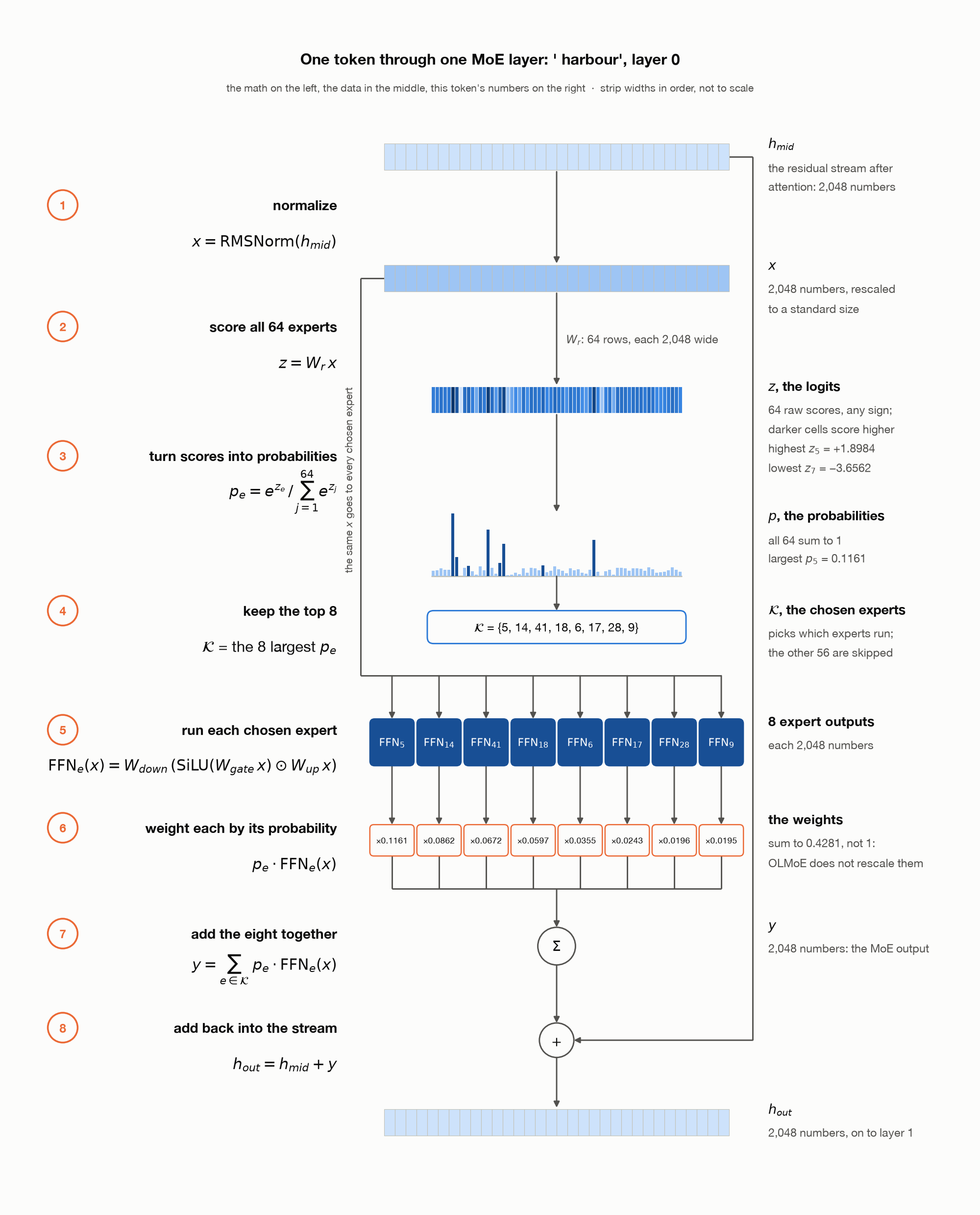
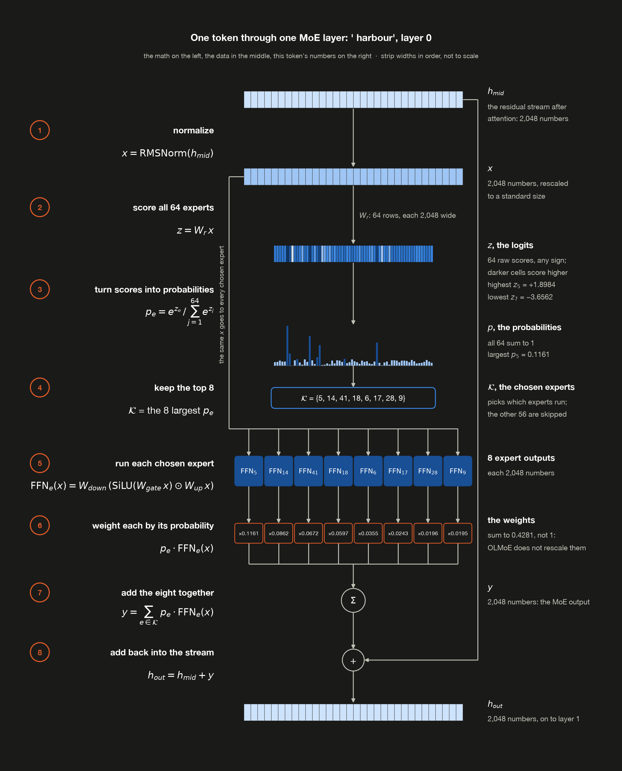
In words: normalize the token’s vector (1), score it against all 64 experts (2), turn the scores into probabilities (3), and keep the eight highest (4). Run those eight experts, each on the same vector (5), scale each output by its probability (6), and add the eight together (7). Finally, add that sum back into the residual stream (8). The other 56 experts never run for this token. The numbers in the figure are the ones in the table below.
Taking the word ' harbour' at layer 0 (one_token_routed):
1
2
3
4
5
6
7
8
9
10
11
12
13
14
15
16
17
18
19
  token                              1 = ' harbour'
  layer                              0
  router output                      64 logits -> softmax -> top-8

  rank  expert    logit  softmax weight
  ---------------------------------------
  1          5  +1.8984          0.1161
  2         14  +1.6016          0.0862
  3         41  +1.3516          0.0672
  4         18  +1.2344          0.0597
  5          6  +0.7148          0.0355
  6         17  +0.3340          0.0243
  7         28  +0.1201          0.0196
  8          9  +0.1143          0.0195

  sum of the 8 kept weights          0.4281
  sum of all 64 weights              1.0000
  discarded by the top-k cut         0.5719
  renormalized? (norm_topk_prob)     no
Add the eight printed weights and you get 0.4281, which is the printed total. That is deliberate: of the 1488 (layer, position) pairs in this passage, 676 reconcile exactly at four decimal places, and the demo pins one of them so a reader who checks the arithmetic finds it correct.
The last line is the part most explanations skip. The softmax runs over all 64 experts and its outputs sum to 1, but only 8 survive the cut, and OLMoE doesn’t rescale them afterwards. The eight weights sum to 0.4281, so 0.5719 of the probability mass is discarded, and the layer’s output is exactly 0.4281 times what it would be if the eight were rescaled to sum to 1.
This is a real design choice with a name in the config, norm_topk_prob, and models differ on it. Setting it true would divide the eight weights by their sum so they add to 1, making every token’s expert mixture equally strong. Leaving it false, as here, lets the router express confidence: a token whose top eight experts are all strongly wanted gets a larger contribution from this layer than a token the router is ambivalent about.
Routing happens independently at every layer, which is easy to miss (routing_depth_profile):
1
2
3
4
5
6
7
8
9
10
11
12
13
14
15
16
17
18
  layer  top-1 expert  its weight  kept total  share
  ----------------------------------------------------
  0                 5      0.1161      0.4281   0.27
  1                53      0.0583      0.2540   0.23
  2                36      0.0866      0.3215   0.27
  3                 0      0.0697      0.3567   0.20
  4                35      0.0761      0.3316   0.23
  5                23      0.0639      0.3003   0.21
  6                17      0.0647      0.3298   0.20
  7                43      0.0443      0.3162   0.14
  8                 6      0.0636      0.3282   0.19
  9                41      0.0540      0.3338   0.16
  10               23      0.1208      0.4334   0.28
  11               55      0.0755      0.3685   0.20
  12               48      0.0764      0.4592   0.17
  13                0      0.0733      0.4784   0.15
  14               46      0.0982      0.4830   0.20
  15               23      0.1158      0.4851   0.24
One word visits sixteen separate committees of eight on its way through the model. There is no such thing as “the expert for ' harbour'”. There are 16 independent choices, and the number of distinct paths a single token could take is astronomically large. Note also that kept total climbs with depth, from 0.25 in layer 1 to 0.49 in layer 15: the router is more decisive in the later layers.
The whole layer, written out
The formula above stops at the MoE output $y$. Two more pieces finish the layer: what each expert computes, and how $y$ rejoins the rest of the model. The new symbols first:
| Symbol | Means | Shape here |
|---|---|---|
| \(h_{mid}\) | the residual stream after attention: the running vector every sub-layer reads from and adds its result back into | $(2048,)$ |
| $\mathrm{RMSNorm}$ | the layer norm OLMoE uses: rescale a vector to unit root-mean-square, then multiply each number by a learned weight; its equation is in the parameter appendix | — |
| \(W_{gate}^{(e)}\), \(W_{up}^{(e)}\) | expert $e$’s two input projections | 1,024 rows × 2,048 wide |
| \(W_{down}^{(e)}\) | expert $e$’s output projection | 2,048 rows × 1,024 wide |
| $\mathrm{SiLU}(u)$ | the activation, $u \cdot \sigma(u)$ where $\sigma$ is the sigmoid, applied to each number separately | — |
| $\odot$ | multiply two vectors number by number | — |
| \(h_{out}\) | what the layer passes to the next one | $(2048,)$ |
Read in order: the $x$ the router scores is a normalized copy of the residual stream; each chosen expert projects it to 1,024 numbers twice, gates one projection by the other, and projects back to 2,048; and the weighted sum $y$ from the first formula is added back into the residual stream.
The demo builds the output for ' harbour' from exactly these equations and compares it with layer 0’s own MoE block (the_layer_by_hand):
1
2
3
4
5
6
7
8
9
10
11
12
13
14
15
  expert  weight p_e  |FFN_e(x)|  |p_e FFN_e(x)|
  ------------------------------------------------
  5           0.1164      0.8041          0.0936
  14          0.0864      0.6428          0.0555
  41          0.0669      1.5089          0.1010
  18          0.0597      0.6144          0.0367
  6           0.0356      1.8434          0.0655
  17          0.0243      0.9634          0.0234
  28          0.0196      0.7652          0.0150
  9           0.0195      0.8227          0.0160

  |y|, sum of the 8 rows (fp32)      0.2074
  |y|, the model's own block (fp32)  0.2074
  largest difference, any coordinate 0.0e+00
  layer output == h_mid + y? (bf16)  yes
Each row is one expert’s contribution, \(p_e\) times its output, and \(\lvert \mathrm{FFN}_e(x) \rvert\) is the length of the output vector, which is how large a change that expert proposes. The eight contributions add up to the model’s own output with no difference at all. That comparison runs in fp32 on a copy of the block, so its weights differ from §3’s bf16 table in the fourth decimal (0.1164 against 0.1161); the last line checks, in the model’s own bf16, that the layer’s output really is the residual stream plus the MoE output.
Expert 41 has only the third-largest weight but makes the largest contribution, because the change it proposes is almost twice as long as expert 5’s. An expert’s influence on a token is its weight times the size of what it proposes, and the router controls only the first.
The same thing in shapes, with the real numbers underneath:
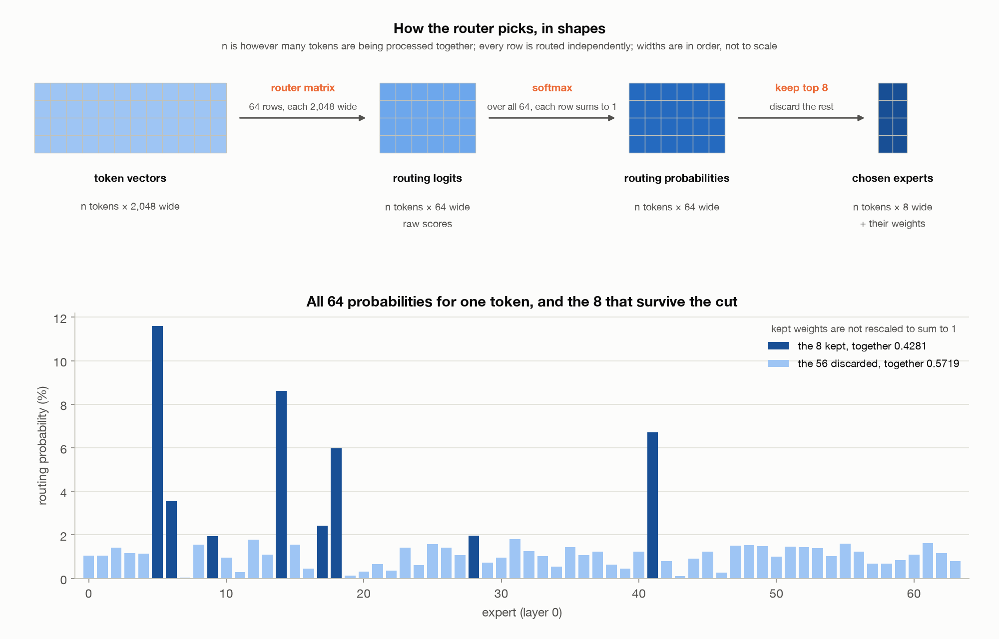
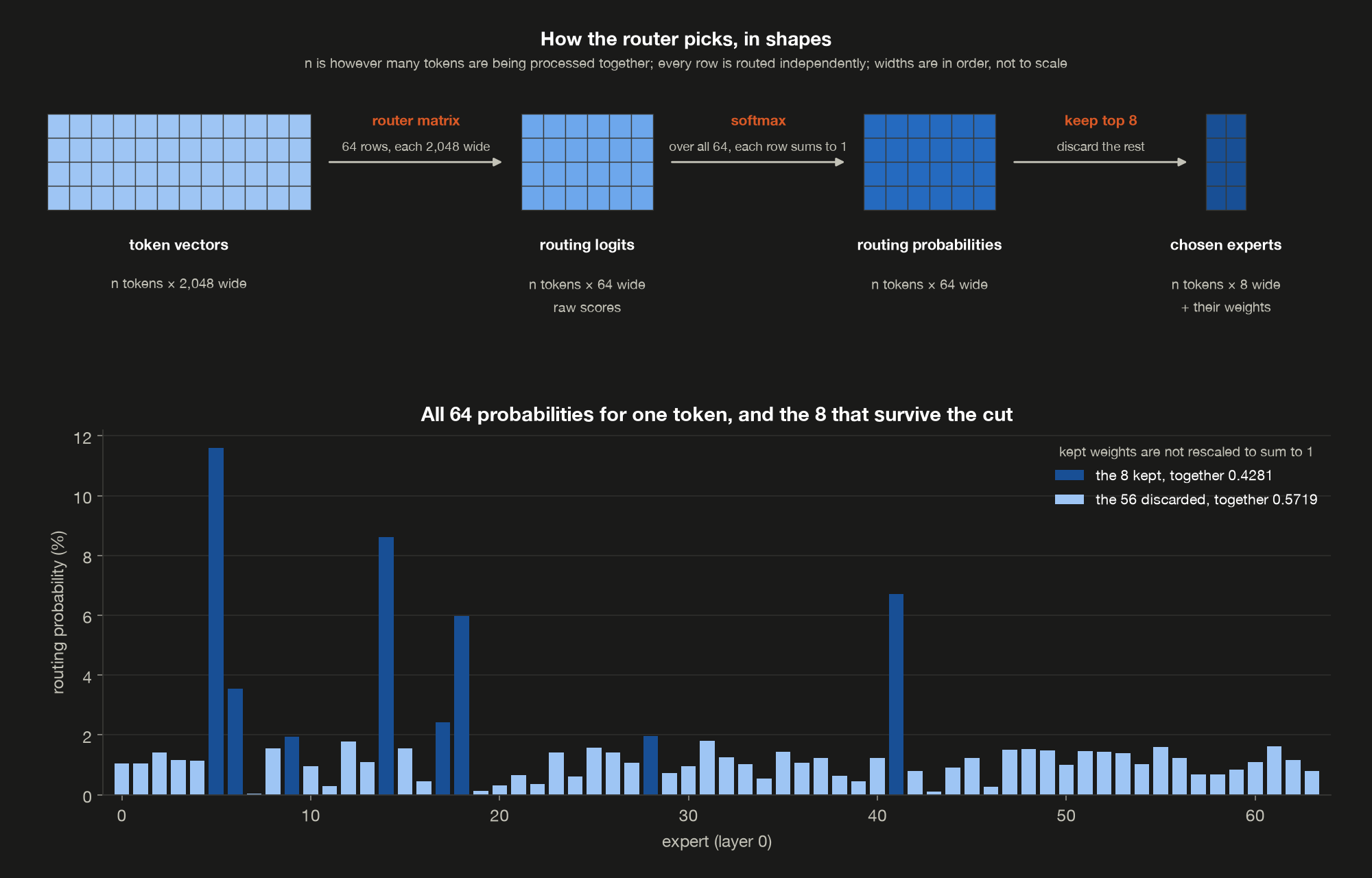
The lower panel shows where the missing 0.5719 went. Eight bars are tall, and the other fifty-six are each small but together larger than the eight. That is what a softmax over sixty-four options looks like when the model has a mild preference rather than a strong one.
Not every router works this way
OLMoE’s router is the plain form, which is why it’s the one to learn first. Nearly every part of it is a decision other models make differently. DeepSeek-V3 makes a different choice on all four. The entries are read from OLMoE’s config and DeepSeek-V3’s config, except the third row’s DeepSeek-V3 entry, which comes from its report (§2.1.2 and §4.2):
| Decision | OLMoE | DeepSeek-V3 |
|---|---|---|
| turning scores into weights | softmax over all 64 | sigmoid per expert: each score squashed to between 0 and 1 on its own, so they need not sum to 1 |
| after the top-k cut | left as-is (norm_topk_prob: false) | rescaled to sum to 1 (true) |
| keeping the load even across experts | an extra training penalty that grows when a few experts get most of the tokens, the auxiliary loss | mainly a per-expert bias nudged during training, plus a much smaller penalty |
| where a token may go | any of the 64 | at most 4 of 8 expert groups |
The third row needs some background, because the problem it addresses isn’t measured until §8. Nothing in the router’s design makes it spread tokens evenly. If it starts sending more tokens to a few experts, those experts get more of the training signal, improve faster and get picked even more, while the others sit mostly idle. The model then pays to store 64 experts and makes real use of only some of them. §8 measures how uneven OLMoE’s routing is, even with a fix in place.
OLMoE’s fix is the auxiliary loss: an extra term added to the training loss that grows when routing is lopsided, so training is pushed toward spreading tokens out. DeepSeek-V3 mostly takes a different route. It keeps one bias number per expert and adds it to that expert’s score when choosing the top 8, but not when computing the weights the chosen experts are multiplied by. After each training step, every overloaded expert’s bias goes down a little and every underused expert’s bias goes up, so tokens drift toward the quiet experts without the loss changing at all. The DeepSeek-V3 report gives the reason: an auxiliary loss large enough to balance the load hurts the model’s quality. It still keeps a small one, weighted 0.0001, as a safeguard against extreme imbalance within a single sequence. OLMoE’s weight is 0.01, a hundred times larger.
The fourth row is about hardware. A model this large has its experts spread over many GPUs, and each token has to be sent to whichever GPUs hold its chosen experts, which §7 measures. DeepSeek-V3 splits its experts into 8 groups, which its report describes as the machines they sit on, and lets each token choose experts from at most 4 of them. That caps how far one token’s work can spread, by construction rather than by luck.
Two more variations you’ll meet in the literature: noisy routing, which adds random noise to the scores during training so the router explores experts it would otherwise never try (Shazeer et al.), and expert capacity, a hard cap on how many tokens one expert may accept per batch, with the overflow either dropped or passed through unchanged (Fedus et al.). Capacity limits exist because of what §8 measures: if the load is uneven and your hardware allocated equal space per expert, something has to give.
4. What the router learns
A common story about MoE models is that experts specialize: one expert becomes good at code, another at French, another at mathematics. But does the router actually send different kinds of text to different experts?
That story is hard to test directly, so this section tests a weaker and more measurable version of it:
If I give the model very different kinds of text, does it route their tokens to different experts?
The demo feeds OLMoE three passages: English prose, Python code, and a paragraph of group theory. For each passage, it records which experts the router selects for every token at every layer.
Remember that OLMoE chooses 8 experts for every token, so a passage of 94 tokens produces 94 × 8 = 752 routing decisions at each layer. I’ll call these routing slots. The three passages aren’t the same length, so they fill different numbers of slots (what_the_router_learns):
1
2
3
4
5
  passage  tokens  routing slots per layer (x 8)
  ------------------------------------------------
  prose        94                            752
  code        140                          1,120
  math        103                            824
We can then ask what share of a passage’s slots went to each of the model’s 64 experts, which are numbered 0 to 63. If an expert receives 60 of prose’s 752 slots, for example, its share is about 8%. Doing that for every expert gives each passage an expert-usage distribution: 64 shares that add up to 100%. Here are five of the 64, in the last layer, layer 15 (what_the_router_learns):
1
2
3
4
5
6
7
8
  expert    prose     code     math
  -----------------------------------
  0         0.66%    0.54%    0.85%
  1         0.00%    4.38%    0.85%
  2         2.53%    0.00%    2.06%
  17        0.13%    9.73%   12.38%
  63        3.06%    0.09%    0.73%
  all 64  100.00%  100.00%  100.00%
Expert 1 gets 4.38% of code’s slots and none of prose’s, and expert 63 leans the other way. If prose and code produce very different distributions across all 64 experts, that’s evidence that the router treats them differently.
How different is “different”?
To put a number on it, I use total variation distance. For each expert, take the difference between the two passages’ shares and ignore its sign; add up the 64 differences, then halve the total. You don’t need the formula to read the results, only the scale: a distance of 0 means two passages used the experts in exactly the same proportions, and a distance of 1 means they had no expert in common at all.
There is one complication, though. Suppose I take two samples of English prose. Even if the router treats them in essentially the same way, 50 tokens from one sample won’t hit the experts in exactly the same proportions as 50 tokens from the other. So a nonzero distance between prose and code doesn’t prove anything by itself. We need to know:
How much difference should we expect even when the kind of text hasn’t changed?
That is the noise floor. The demo estimates it by splitting each passage in half, measuring the distance between the two halves of the same passage, and averaging over the three passages. The halves are shorter than the full passages, and shorter samples differ more by chance, so if anything this floor is set high, which makes the comparison harder to pass rather than easier.
Here is every layer. noise is the noise floor, the next three columns are the pairs of different passages, cross is the average of those three, and the last column divides cross by noise (what_the_router_learns):
1
2
3
4
5
6
7
8
9
10
11
12
13
14
15
16
17
18
19
20
21
22
23
  layer  noise  prose/code  prose/math  code/math  cross  cross/noise
  ---------------------------------------------------------------------
  0      0.240       0.465       0.362      0.371  0.400         1.7x
  1      0.227       0.524       0.380      0.346  0.416         1.8x
  2      0.254       0.595       0.476      0.345  0.472         1.9x
  3      0.222       0.616       0.459      0.356  0.477         2.1x
  4      0.235       0.694       0.551      0.345  0.530         2.3x
  5      0.232       0.772       0.631      0.320  0.574         2.5x
  6      0.213       0.769       0.627      0.349  0.581         2.7x
  7      0.224       0.772       0.628      0.354  0.585         2.6x
  8      0.210       0.736       0.508      0.491  0.578         2.7x
  9      0.216       0.847       0.559      0.435  0.613         2.8x
  10     0.204       0.803       0.475      0.436  0.571         2.8x
  11     0.200       0.854       0.553      0.385  0.597         3.0x
  12     0.206       0.818       0.532      0.409  0.586         2.8x
  13     0.197       0.812       0.631      0.505  0.649         3.3x
  14     0.210       0.759       0.586      0.409  0.585         2.8x
  15     0.173       0.855       0.596      0.505  0.652         3.8x
  mean   0.216       0.731       0.535      0.397  0.554        2.56x

  noise floor, mean over layers      0.216
  cross-domain, mean over layers     0.554
  cross-domain over noise floor      2.56x
The mean row is the first result. Two halves of the same text differ by 0.216 on average. Two different kinds of text differ by 0.554, which is 2.56× the noise floor. So the router’s expert choices clearly depend on the kind of text.
That does not yet mean there’s a “code expert” or a “math expert”. It only tells us that code, prose and mathematics produce measurably different routing patterns.
The difference grows deeper in the model
The rows show a second pattern. Taking the first and last layers out of that table (what_the_router_learns):
1
2
3
4
5
                         layer 0  layer 15
  ------------------------------------------
  noise floor              0.240     0.173
  cross-domain distance    0.400     0.652
  cross-domain / noise      1.7x      3.8x
At layer 0, different kinds of text are only 1.7× farther apart than the noise floor. By layer 15 they’re 3.8× farther apart. Two things happen at once. The noise floor falls from 0.240 to 0.173, so two halves of the same text route more alike, while the cross-domain distance rises from 0.400 to 0.652, so different kinds of text route less alike. The climb in between isn’t smooth (layer 13 jumps to 3.3× and layer 14 falls back to 2.8×), but the last column stays under 2× for layers 0 to 2 and is 2.8× or more from layer 9 onward.
So deeper in this model, routing becomes more consistent within a kind of text and more different across kinds. One possible interpretation is that early routing responds to surface features such as individual tokens, punctuation and formatting, while later layers route on richer representations of what the text is about. That is an interpretation, though, not something this experiment proves.
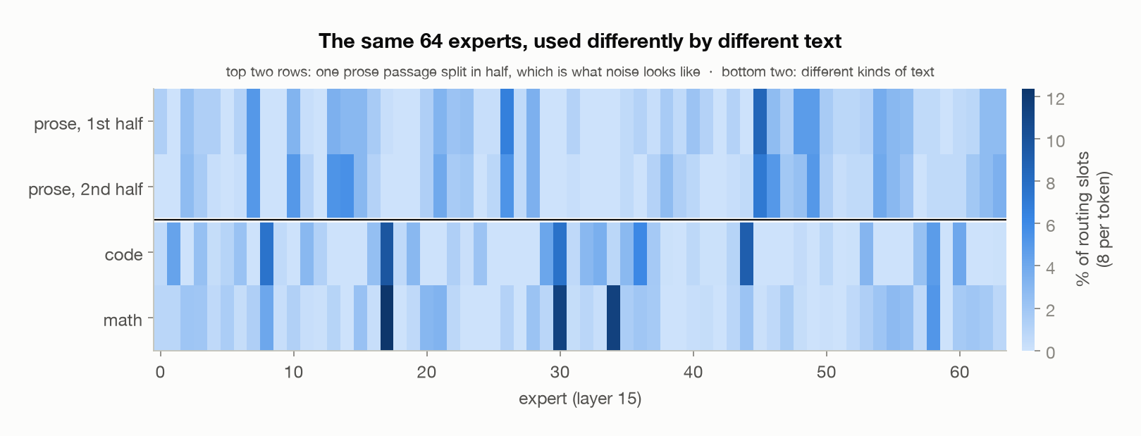
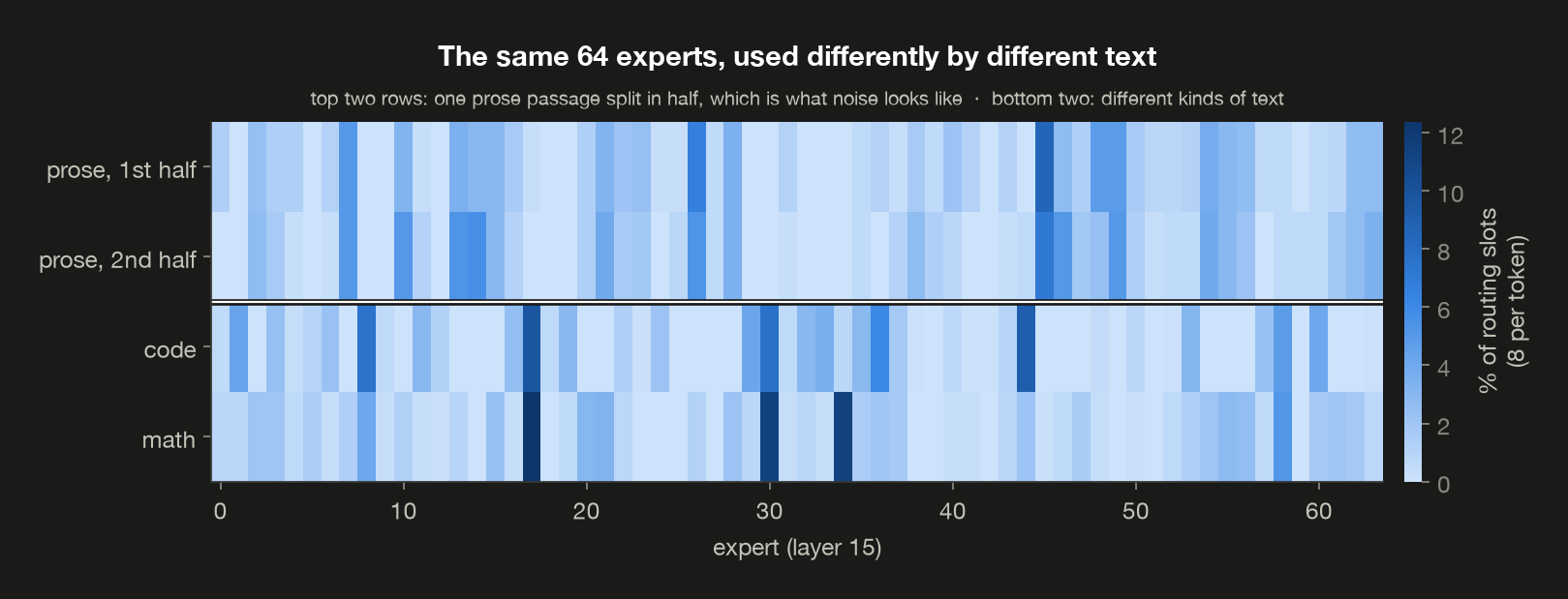
The top two rows are the same prose passage split in half; the bottom two are code and mathematics. The comparison to make by eye is row 1 against row 2 (noise) versus row 1 against row 3 (signal).
Some individual experts show striking preferences
A distance sums up all 64 experts at once, and single experts can be far more lopsided. The expert whose share rises most between prose and code in layer 15 (what_the_router_learns):
1
2
3
4
5
6
  expert                             17
    code slots it received           109 of 1,120 = 9.73%
    prose slots it received          1 of 752 = 0.13%
    math slots it received           102 of 824 = 12.38%
    an even share would be           1.56%
  experts code uses, prose never     13
Expert 17 receives 109 of code’s 1,120 slots (9.73%) and 1 of prose’s 752 (0.13%), where an even share would be 1.56%. Thirteen experts are used by code and never by prose.
It is tempting to look at that and say: expert 17 is a code expert. Its own block argues against that. It takes an even larger share of the mathematics passage, 102 of 824 slots (12.38%), so whatever expert 17 responds to, it isn’t code as such.
Different routing doesn’t necessarily mean specialized experts
The experiment above shows something real: code, English prose, and mathematics take different routes through OLMoE.
But does that mean we have found a “code expert,” an “English expert,” and a “math expert”?
Not necessarily.
Imagine that Python code frequently gets sent to experts 3, 29, and 42, while English prose gets sent to experts 8, 21, and 55. From that observation, we know that the router treats the two inputs differently. But we still don’t know what those experts actually do.
An expert might genuinely perform some computation that is especially useful for code. Or it might respond to patterns that simply occur more often in code: punctuation, indentation, particular token combinations, or some feature that doesn’t have a neat human-readable name. The real expert 17 above is a warning about exactly this. It looked like a code expert until we checked mathematics, where it took an even larger share.
That gives us three different claims:
Different inputs get different routing. This is what our experiment shows. Code, prose, and mathematics produce measurably different mixtures of experts.
Different experts do meaningfully different things. That’s plausible, but our routing counts don’t show it. We know which experts ran, not what each one contributed.
A particular expert has a recognizable skill. This is the strongest claim: “expert 17 is a coding expert.” Our experiment definitely can’t establish that.
So how could we get stronger evidence?
Instead of just observing expert 17, we could intervene. Turn it off and run the model again.
If coding performance suddenly gets much worse while ordinary prose is mostly unaffected, that’s evidence that expert 17 performs something particularly important for code. If almost nothing changes, perhaps other experts can easily replace it.
Counting where tokens go tells us about routing. Changing where they go and measuring what breaks tells us much more about function.
Why different text might route differently anyway
There is another reason to be careful about interpreting our results.
The router doesn’t literally read a token and think:
“This is Python. Send it to the coding expert.”
By the time a token reaches an MoE layer, the transformer has already turned it into a hidden state: a long list of numbers representing what the model has learned about that token in its current context.
One useful mental model is to imagine these hidden states as points on a giant map. Tokens represented similarly by the model tend to occupy nearby regions of this map.
The router makes its decision from that hidden state.
So suppose code and English prose already occupy different regions of the model’s representation space. Even without cleanly specialized “code” and “English” experts, the router could naturally send them toward different experts.
This is the argument Wang, Hayou and Nalisnick make in The Myth of Expert Specialization in MoEs (2026). They show it mathematically, and the reason is the router itself: it is the single linear map from §2 and nothing more. Their Proposition 1 makes the consequence precise: tokens with similar representations must receive similar routing scores.
The reverse is not guaranteed. Two very different hidden states can still end up using similar experts.
That changes how we should interpret plots of expert usage.
A plot showing that code and prose activate different experts might look like a map of specialized skills. But it could instead be revealing something simpler: the model already represents code and prose differently, and the router is responding to that difference.
In fact, the paper specifically points to OLMoE’s own expert-specialization figure (Figure 22 of Muennighoff et al.) as an example of evidence that should be interpreted carefully.
This doesn’t mean experts aren’t specialized. It means routing patterns alone aren’t enough to prove that they are.
What happens when researchers actually intervene?
Researchers have also tried the stronger experiment: change the experts and see what happens.
The results are more complicated than either “every expert has its own skill” or “experts are all interchangeable.”
For example, Wang, Hayou and Nalisnick prune away all but the twelve most-used experts in the last layers of one model. When the model is only processing the prompt, removing the final two layers’ worth barely changes the loss. That might make the removed experts look unnecessary.
But once the model starts generating new tokens, removing those experts hurts much more.
So experts that looked unimportant from their activation patterns were actually useful under a different workload.
Other work tries to measure the causal contribution of individual experts more directly. Hu et al., in What Gets Activated (2026), study this question using causal effects rather than routing frequency alone.
One picture emerging from this line of research is more nuanced than the simple “one expert = one skill” story. A relatively small core set of experts may handle much of the traffic across many domains, while more specialized behavior appears in a surrounding set of less frequently used experts.
So the architecture may look less like:
coding expert + math expert + French expert + reasoning expert
and more like:
shared general-purpose experts + some experts that become more important for particular kinds of inputs.
There’s one more wrinkle: depth
Our OLMoE experiment found that code, mathematics, and prose become more differently routed in later layers.
Wang, Hayou and Nalisnick observe the opposite pattern in some of the models they study: unrelated prompts can converge toward nearly identical expert usage in deeper layers.
That sounds contradictory, but the experiments aren’t identical.
Their models are larger and deeper than OLMoE’s 16 layers, so “deep” doesn’t necessarily mean the same thing. More importantly, they find that this convergence happens during prefill (the initial pass where the model reads the prompt) and can reverse once the model begins decoding, generating one new token at a time (post 2 §6).
Our experiment only measures that first part: one prefill pass over fixed text. We don’t generate any new tokens.
That makes the disagreement interesting rather than something we need to explain away. Different models, layers, and phases of inference can produce different routing behavior.
So what did we actually learn?
We can confidently say:
Code, mathematics, and English prose travel through OLMoE differently.
We can measure those differences, and we can see how they change across layers.
What we cannot conclude from those measurements is that expert 17 “knows code” or expert 42 “knows mathematics.”
To make claims like that, we’d need to go beyond watching where tokens travel. We’d need to intervene on individual experts and measure what actually changes in the model’s behavior.
Routing tells us where a token went. It doesn’t, by itself, tell us what the expert knows.
5. Two bills: memory and time
“1B active, 7B total” describes two costs that behave completely differently, and confusing them is an easy practical mistake to make with these models. Both bills come from numbers we already have, so this section is mostly arithmetic you can follow line by line.
Memory is billed on total parameters. Every expert has to be resident, because the router decides at run time and any token might want any of them. There’s no subset you could have left on disk.
Turning that into gigabytes takes two steps. Every parameter is stored in bfloat16, which is 2 bytes each, so the model’s bytes are its parameter count doubled. Then a GiB is $1{,}073{,}741{,}824$ bytes, which is $2^{30}$, so dividing by that gives the figure a memory budget is written in (two_bills):
1
2
3
4
5
6
7
  Memory is billed on every parameter, run or not:

  step                                    result
  ------------------------------------------------------------
  parameters in the model          6,919,161,856  parameters
  x 2 bytes each (bfloat16)       13,838,323,712       bytes
  / 1,073,741,824 bytes in a GiB           12.89         GiB
12.89 GiB for a model whose name starts with “1B”. The parameter count on the first row is §1’s census, unchanged.
Time is billed on active parameters. The way to see that is to leave everything else alone and change only $k$, the number of experts each token is routed to. Only the expert term moves when $k$ does, and it moves in proportion: one expert is 6,291,456 parameters, eight of them is eight times that, and all 64 is sixty-four times it. So going from $k = 8$ to $k = 64$ is exactly 8× the expert arithmetic:
1
2
3
4
5
6
  step                             result
  -----------------------------------------------------
  one expert                    6,291,456  parameters
  x 8 chosen per token         50,331,648  parameters
  x 64 if every expert ran    402,653,184  parameters
  ratio of expert arithmetic           8x
That is the prediction. Now the measurement. Same weights, same memory, $k$ raised from 8 to 64, and the forward pass timed (two_bills):
1
2
3
4
5
6
7
8
  experts per token  forward (ms)  vs top-8
  -------------------------------------------
  8                         439.7     1.00x
  64                        932.2     2.12x

  expert arithmetic ratio            8x
  measured wall-clock ratio          2.12x
    below 8x because attention, norms and the LM head are unchanged
Eight times the expert arithmetic costs 2.12× the wall clock, and zero extra bytes of weights.
The gap between 8× and 2.12× is the whole point. Only the expert multiplies grew. Attention, the norms and the LM head did exactly as much work in both runs, and on a 94-token forward pass they’re a large share of the total, so they dilute the part that octupled. That’s why “active parameters” predicts the trend of speed and not a clean multiplier: the number is real, but what it scales is one term out of several.
Two warnings about that table. Unlike every other number in this post, these are wall-clock measurements and they move a little from run to run; the counts and ratios elsewhere don’t. And the top-64 row measures cost only. Because norm_topk_prob is false, routing to all 64 experts changes what the model computes, so it’s a timing experiment, not a quality one.
Put the two bills together and you get the practical warning. The model is not a drop-in replacement for either dense model its name suggests:
1
2
3
4
5
6
7
  step                        result
  ------------------------------------------------
  resident parameters  6,919,161,856  parameters
  active parameters    1,178,994,688  parameters
  resident / active            5.87x
    so it needs 5.9x the memory of a dense model
    its active size, while doing a fraction of a 6.9B model's work
Against a 1B dense model it needs about 5.9 times the memory, which is the resident count divided by the active one. Against a 7B dense model it does a fraction of the arithmetic, so it isn’t that either. What it buys is the quality that comes with more parameters at close to the speed that comes with fewer, and it pays for that in RAM.
6. Sparsity does not survive a batch
Of everything in this post, this is the result I found least obvious.
Every claim so far has been about one token. One token uses 8 of 64 experts. But nothing is served one token at a time: you process a prompt of hundreds of tokens at once, and you batch requests from many users together. So the question that decides real cost is: how many distinct experts does a group of tokens need between them?
Each token picks its own 8. If two tokens pick differently, the hardware has to touch the union of their choices.
Measuring that takes one decision worth spelling out, because it’s what makes the numbers below look odd at first. Cut the passage into consecutive blocks of the size you care about, two tokens at a time, then four, and so on, and count the distinct experts each block needs between them. Every layer routes independently, so each block yields 16 counts rather than one, and the table averages all of them. That’s why a column headed “experts needed” holds 13.1: it’s a mean over blocks and layers, not a count of any particular block. The “of 64” column is that mean as a share of the experts there are, and the last column is simply the block size times 8, the routing slots those tokens fill (batch_collapse):
1
2
3
4
5
6
7
8
9
10
11
12
13
14
15
16
  passage                            356 tokens, English prose

  tokens together  experts needed  of 64  expert-slots used
  -----------------------------------------------------------
  1                           8.0    12%                  8
  2                          13.1    20%                 16
  4                          21.1    33%                 32
  8                          31.4    49%                 64
  16                         40.8    64%                128
  32                         48.5    76%                256
  64                         53.9    84%                512
  128                        58.0    91%               1024
  256                        60.9    95%               2048
    'experts needed' is a mean over consecutive blocks of that size
    and all 16 layers, so it is not a whole number.
    'expert-slots used' is the block size x 8.
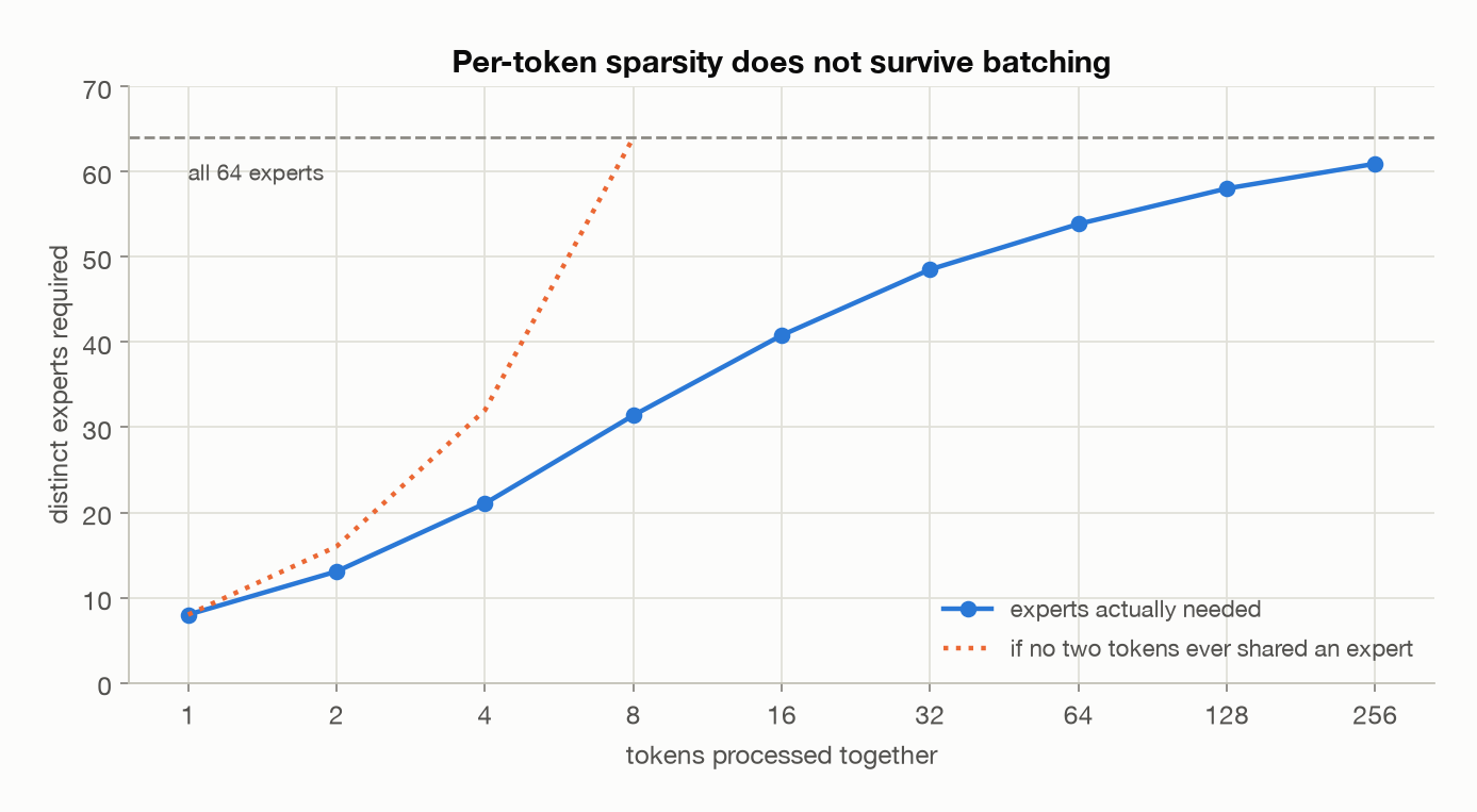
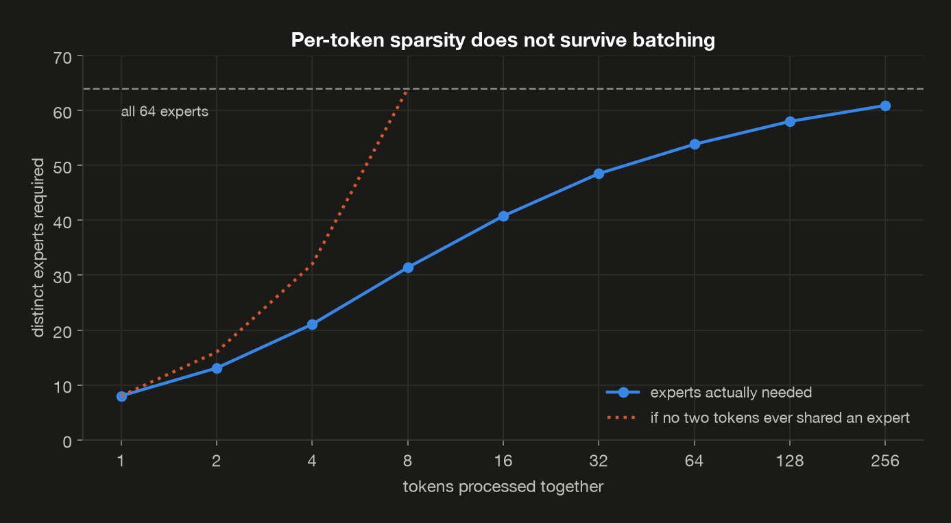
Eight tokens already need half the experts. Two hundred and fifty-six need 60.9 of 64, which is 95%.
So the sparsity that makes an MoE cheap is a property of a token, and it evaporates the moment you process tokens together. The dotted line on the chart is the worst case, where no two tokens ever share an expert; it reaches all 64 by eight tokens. The measured curve sits below it because these tokens do share experts, but not far enough below to change the conclusion. At any realistic batch size essentially every expert is needed by somebody, so the residency §5 described stops being a precaution against an unlucky token and becomes the ordinary case.
One passage flatters the result
That curve came from a single passage of English prose, and §4 is reason enough to distrust it. If different kinds of text route differently, a batch that mixes them should need more of the experts, not fewer. Real batches mix them constantly: your prompt and a stranger’s go through the same forward pass.
So measure it instead of assuming it. Three passages are routed as separate requests and interleaved into one batch, once from three parts of the same prose and once from the prose, code and mathematics of §4. Both batches are assembled identically and take 94 tokens from each passage, so the domain mix is the only thing that differs (batch_composition):
1
2
3
4
5
6
7
8
9
10
11
12
  tokens from each passage           94

  tokens together  one domain  three domains  difference
  --------------------------------------------------------
  2                      14.1           14.7        +0.5
  4                      22.4           23.7        +1.4
  8                      32.4           34.9        +2.5
  16                     42.2           46.6        +4.4
  32                     49.9           55.3        +5.4
  64                     55.5           60.2        +4.8
  128                    59.0           62.3        +3.2
  256                    61.5           63.7        +2.2
Mixing domains costs more experts at every size. The gap is widest at 32 tokens together, where three domains need 55.3 of 64 against one domain’s 49.9, and by 256 tokens the mixed batch reaches 63.7 of 64, which is 99.5%.
That is worth saying plainly, because it runs the opposite way from the usual caveat about measuring on one text: the headline number above is conservative. A single passage understates how fast sparsity disappears, and §4’s specialization is exactly why. The same routing differences that make the per-token saving real make the per-batch saving worse.
That is what “1B active, 7B total” means in practice. An MoE saves arithmetic, not memory. Per token, 17% of the parameters multiply. Per batch, essentially 100% of them have to be in RAM and get read. That connects to post 2’s finding that generating a token is limited by memory bandwidth rather than arithmetic. For a single token an MoE reads only its eight experts, which is why it generates quickly; for a batch it reads nearly all of them, so at serving batch sizes the bandwidth saving mostly disappears.
How a batch is computed
Written per token, a batch of $T$ tokens is $T$ separate copies of the layer formula. With $\mathbf{1}[\cdot]$ meaning 1 when the condition inside holds and 0 otherwise:
\[y_t = \sum_{e=1}^{64} \mathbf{1}[e \in \mathcal{K}_t]\; p_{t,e}\; \mathrm{FFN}_e(x_t) \qquad \text{for each token } t = 1, \dots, T\]Nobody computes it that way. Swapping the order of the two sums groups the work by expert instead of by token. For each expert $e$, collect the tokens that chose it, \(T_e = \{t : e \in \mathcal{K}_t\}\), stack their vectors into one matrix, run \(\mathrm{FFN}_e\) on all of them in a single matrix multiply, scale each result by that token’s \(p_{t,e}\), and add it back to its own token. OLMoE’s implementation in transformers is this loop over experts. At layer 0, for the 356-token passage (batch_collapse):
1
2
3
4
5
  experts called                     64 of 64
  tokens per call, fewest            1
  tokens per call, median            39
  tokens per call, most              254
  tokens x 8 routing slots           2,848
All 64 experts are called, which is this section’s finding seen from the hardware’s side, and the calls are very uneven: one expert multiplies a single token while another multiplies 254. Uneven call sizes are what the expert capacity limits in §3 exist to bound, and across several GPUs they’re what makes §7’s traffic uneven too.
7. When the model spans many GPUs
Everything so far assumed the model fits on one machine. OLMoE does, at 12.89 GiB. The models this architecture exists for don’t: DeepSeek-V3 has 671B parameters, over a terabyte of weights in bf16, so it has to be split across many GPUs.
There are two ways to split a transformer across machines, and MoE makes the second one natural.
Tensor parallelism cuts the matrices themselves. Take one weight matrix, slice it into as many pieces as you have GPUs, and give each GPU a piece. Every GPU then sees every token and multiplies it by the slice it holds, so each ends up with a partial result: a piece of the answer, correct as far as it goes but missing the contributions of every other slice. Those partials have to be added together before the layer can continue, and that sum is a collective operation called an all-reduce, in which every GPU sends its partial to all the others and comes away with the total. A transformer layer pays for one after attention and one after the FFN.
Expert parallelism cuts along the experts instead, leaving every matrix whole. GPU 0 gets experts 0 to 7, GPU 1 gets experts 8 to 15, and so on. Nothing needs slicing, because the experts were already separate objects: no arithmetic in an MoE layer ever crosses from one expert to another, so the seam is already there in the model. What travels now is not partial results but the tokens themselves. A token has to be sent to each GPU holding one of its chosen experts, and the outputs sent back, which is the all-to-all exchange described above, twice per MoE layer.
The difference that matters in practice is what decides the bill:
| tensor parallelism | expert parallelism | |
|---|---|---|
| what gets split | every matrix, along one dimension | the experts, each kept whole |
| what moves between GPUs | partial results, all-reduced | tokens, all-to-all |
| how much moves | fixed by the model’s shape | decided by the router, per token |
| is the load even? | yes, by construction | only if the router cooperates |
Tensor parallelism is predictable. Its communication is the same on every batch, because it follows from the shape of the matrices and nothing else, and every GPU does an equal share of the arithmetic. Expert parallelism is contingent. Its communication depends on where the router happens to send things, which is what the table above measures, and its load depends on whether the experts are evenly popular, which §8 shows they are not.
In practice these aren’t rival choices so much as tools for different parts of the same model, and a real deployment uses both at once. DeepSeek-V3’s report (§3.4) describes serving it on 32 GPUs for prefill, with attention on 4-way tensor parallelism and the MoE layers on 32-way expert parallelism, and on 320 GPUs for decoding, where the MoE part is 320-way expert-parallel and each GPU holds a single expert. Attention has no expert seam to exploit, so it gets tensor parallelism; the MoE part has nothing else that splits so cleanly, so it gets expert parallelism. The report also notes that they keep redundant experts, extra copies of the busiest ones, rearranged between GPUs according to the load actually observed, which is §8’s imbalance turning into a hardware countermeasure. During training they avoided tensor parallelism altogether, calling it costly.
The catch follows directly from §6. Routing is per token, and a token’s eight experts are wherever the router says they are. If those eight live on five different GPUs, that token has to be sent to five GPUs and its results gathered back, at every layer and for every token. That exchange is the all-to-all, and it’s one of the central engineering problems in serving MoE models.
How much traffic that is depends entirely on how scattered the routing is, and that’s measurable from the routing indices alone, without owning a single GPU.
The arrangement is the simple one expert parallelism uses: deal the 64 experts out in contiguous blocks, so at four GPUs the first holds experts 0 to 15, the second 16 to 31, and so on. Then take one token at one layer, look at where its eight experts landed, and count the distinct GPUs among them. Averaging that over every token and all 16 layers gives the GPUs per token column. Of all is that average as a share of the GPUs there are, and tokens needing all is how often a token’s eight experts reach every GPU in the machine (experts_across_gpus):
1
2
3
4
5
6
7
8
9
10
11
12
  passage                            356 tokens, English prose

  GPUs  experts each  GPUs per token  of all  tokens needing all
  ----------------------------------------------------------------
  2               32            1.99    100%                 99%
  4               16            3.67     92%                 68%
  8                8            5.54     69%                  0%
  16               4            6.84     43%                  0%
    experts are dealt to GPUs in contiguous blocks, as expert
    parallelism does. 'GPUs per token' counts the distinct GPUs one
    token's 8 experts land on, averaged over every token and
    all 16 layers; 'of all' is that as a share of the GPUs there are.
Split across four GPUs, the average token needs 3.67 of them, and 68% of tokens need all four. At two GPUs, 99% of tokens need both; the router almost never keeps a token’s work on one side.
The number of GPUs a token needs climbs while the share falls. Going from 8 GPUs to 16 raises the GPUs a token must reach from 5.54 to 6.84, so each token’s work is spread thinner and communicated wider. It can’t exceed 8, because a token only picks 8 experts, which is why the “of all” column drops. This is §6’s finding again, counted in GPUs: a token’s choices are scattered, so nothing about them stays local.
What this section does and does not measure. The routing is real, measured on the actual model. The GPU assignment is arithmetic on top of it, not a benchmark on a multi-GPU host, which isn’t something a laptop can honestly produce. What it gives you is the quantity that determines the communication cost, rather than the cost itself, which depends on the serving stack and on interconnect bandwidth: how fast the links between GPUs can carry data, as distinct from how fast the GPUs compute.
For scale, here is how OLMoE sits next to two models built the same way. These are published values rather than measurements of mine, from each model’s configuration (OLMoE, Qwen3-30B-A3B, DeepSeek-V3) and, for the active counts, each model’s name or report:
| OLMoE-1B-7B | Qwen3-30B-A3B | DeepSeek-V3 | |
|---|---|---|---|
| total parameters | 6.9B | 30.5B | 671B |
| active per token | 1.2B | ~3B | 37B |
| layers | 16 | 48 | 61 |
| routed experts per layer | 64 | 128 | 256 |
| experts per token | 8 | 8 | 8 |
| shared expert | none | none | 1, always on |
| fits on one 24 GB card | yes, in bf16 | no | not remotely |
Two details in that last column are often drawn wrong in simplified diagrams of DeepSeek-V3, and both are stated in its report, §4.2. It has a shared expert that every token passes through in addition to its top-8, so “8 of 256” understates what runs. And its first three layers are ordinary dense FFNs, not MoE layers, so it has 58 MoE layers rather than 61. Its experts are also much narrower than its dense layers (an intermediate width of 2,048 against the 18,432 of the dense FFN), which is what lets it hold 256 of them per layer.
8. Nothing balances the load for free
One more consequence of letting a learned component do the choosing: nothing makes the experts equally popular.
There is a degenerate outcome sitting in this architecture. If the router slightly prefers a few experts early in training, those experts get more of the gradient (the signal that says which way to nudge each weight to reduce the error), so they improve faster, get preferred more strongly, and the rest starve. You would end up paying for 64 experts and effectively training a handful.
The last column below is the coefficient of variation, the standard deviation of expert usage divided by its mean: a scale-free measure of unevenness where 0 is perfectly even and around 1.0 means the spread between experts is about as large as the average usage itself. Measured over the same prose passage’s 2,848 routing slots per layer (load_balance):
1
2
3
4
5
6
7
8
9
10
11
12
  passage                            356 tokens, English prose
  routing slots per layer            2848

  layer  busiest  quietest  busiest vs even  coeff of var
  ---------------------------------------------------------
  0        8.92%     0.04%            5.71x          0.88
  8        7.30%     0.00%            4.67x          0.89
  15       8.32%     0.00%            5.33x          1.07

  even share would be                1.56%
  router_aux_loss_coef               0.0100
  experts never used (last layer)    4
An even share would be 1.56%. The busiest expert in layer 0 takes 8.92%, which is 5.71× that, while the quietest takes 0.04% and four experts in the last layer are never used by this passage at all. (That count is a property of this passage, not of the model: it’s one domain, and §6 measured what happens when a batch stops being one domain. A broader sample uses more of them.)
This is why MoE training carries auxiliary losses: extra penalty terms added to the training objective. OLMoE’s objective has three terms (Muennighoff et al., §2):
| Symbol | Means |
|---|---|
| \(\mathcal{L}_{CE}\) | cross-entropy, the ordinary next-token loss: averaged over tokens, $-\log$ of the probability the model gave the token that actually came next |
| \(\mathcal{L}_{LB}\) | the load-balancing loss, large when a few experts take most of the traffic |
| \(\mathcal{L}_{RZ}\) | the router z-loss, large when the router’s logits grow large |
| $\alpha$, $\beta$ | how much each penalty counts; for OLMoE-1B-7B, 0.01 and 0.001 |
The two penalties need a few more quantities, each averaged over the $N$ token positions in a batch:
| Symbol | Means | Sums to |
|---|---|---|
| \(N_E\) | the number of experts | 64 |
| \(f_i\) | the fraction of tokens that have expert $i$ among their top 8 | 8, over all experts |
| \(P_i\) | the router probability given to expert $i$, averaged over tokens | 1, over all experts |
| \(z_{t,j}\) | token $t$’s router logit for expert $j$ | — |
If routing were perfectly even, every \(f_i\) would be $8/64$ and every \(P_i\) would be $1/64$, so \(\mathcal{L}_{LB} = 64 \times 64 \times \tfrac{8}{64} \times \tfrac{1}{64} = 8\). It grows when the experts picked most often are also the ones given the most probability, which is what a router locking onto a few experts looks like. One detail matters for how it trains: \(f_i\) is a count of top-8 selections, so like the selection itself it has no gradient. Only \(P_i\) does, and through it the loss pushes probability away from experts that are already taking more than their share.
The z-loss squares the logarithm of the softmax’s denominator. Keeping it small keeps the router’s logits in a range where the softmax stays numerically stable, which is the reason the paper gives for it.
On the 94-token passage (what_training_minimizes):
1
2
3
4
5
6
7
8
9
10
11
12
13
14
15
16
17
  tokens scored                      93 (each predicts the next)
  L_CE, cross-entropy                2.7381

  sum of f_i over experts            8.0000
  sum of P_i over experts            1.0000
  L_LB if routing were even          8.0000
  L_LB by hand, all layers pooled    8.1675
  L_LB, transformers' own function   8.1675
  L_LB by hand, mean of per-layer    10.5038
  L_RZ, router z-loss (paper)        11.5881

  term           coefficient    value  contribution
  ---------------------------------------------------
  L_CE                     1   2.7381        2.7381
  L_LB (pooled)         0.01   8.1675        0.0817
  L_RZ                 0.001  11.5881        0.0116
  total                                      2.8314
The sums come out at 8 and 1, as the definitions require, and the hand computation equals transformers’ own function. The pooled value, 8.17, looks almost perfectly balanced, and that’s partly an artifact. transformers’ function pools the router logits of all 16 layers before counting, which treats expert 5 in layer 0 and expert 5 in layer 15 as one expert and averages each layer’s imbalance away; computed layer by layer, the same passage scores 10.50. transformers adds only \(\alpha\,\mathcal{L}_{LB}\) to the loss it returns, so the z-loss here comes from the paper’s formula, shown for scale.
Weighted by their coefficients, the two penalties add 0.0817 and 0.0116 to a cross-entropy of 2.7381, about 3% and 0.4%. That is small on purpose: the balancing term is there to stop a collapse, not to drive the model, and setting it too high would trade away prediction quality to make a histogram look tidy. Even with that penalty applied throughout training, the busiest expert still runs about five times as often as an even share. The auxiliary loss keeps the distribution from collapsing; it doesn’t make it flat.
What’s left over stops being a training concern and becomes a hardware one, which is where §7 comes back. If the busiest expert runs five times as often as an even share, the GPU holding that expert does five times the work, and the whole batch waits for it. DeepSeek-V3’s report (§3.4) describes the countermeasure: it serves redundant experts, extra copies of the busiest ones, so that each of the 32 GPUs in a prefill unit holds one spare on top of its eight, and it rearranges which experts sit where according to the load it actually observes in production. The balancing loss narrows the distribution during training. Whatever survives, the serving stack pays for.
9. How an MoE is trained, and where “mid-training” fits
Two different things often get talked about in the same breath here: mixture-of-experts is an architecture, while pre-training, mid-training and post-training are stages in a model’s life. They are different dimensions, not alternatives. You can ask “is this model MoE?” and “what stage is it in?” independently.
The experts and the router learn together, during pre-training. They aren’t bolted on afterwards. At the start of training every expert is random and the router is random, so the first routing decisions are meaningless. Then ordinary next-token prediction runs: the model reads text, predicts what comes next, and is scored on how wrong it was. Backpropagation then works that error backwards through the network to get a gradient for every weight involved, and the weights move. The router, the chosen experts and the rest of the network all update. The skipped experts don’t, because they contributed nothing to the output.
There is a subtlety here that §3 set up. Picking the top 8 is a discrete choice, and discrete choices have no useful gradient: you can’t differentiate “expert 5 was ranked higher than expert 6”. So how does the router learn anything at all? Through the weights \(p_e\) that multiply each expert’s output. Two symbols first, then the chain rule:
| Symbol | Means |
|---|---|
| \(g_e\) | how much the loss would change if expert $e$’s output grew along its own direction: \(g_e = \frac{\partial \mathcal{L}}{\partial y} \cdot \mathrm{FFN}_e(x)\), one number per chosen expert |
| \(\delta_{ej}\) | 1 if $e = j$, and 0 otherwise |
Treat the chosen set $\mathcal{K}$ as fixed, differentiate \(y = \sum_{e \in \mathcal{K}} p_e\,\mathrm{FFN}_e(x)\) through the softmax, and for every expert $j$:
\[\frac{\partial \mathcal{L}}{\partial z_j} = \sum_{e \in \mathcal{K}} g_e\; p_e\,(\delta_{ej} - p_j) \qquad \frac{\partial \mathcal{L}}{\partial W_r} = \frac{\partial \mathcal{L}}{\partial z}\, x^{\top}\]Two consequences follow:
- Every router row gets a gradient, not only the eight chosen ones. The \(-p_j\) term is present for all 64, because each \(p_e\) has every expert’s score in its denominator: raising a chosen expert’s probability means lowering everyone else’s.
- Only the chosen experts’ own weights get a gradient. A skipped expert’s FFN never appears in $y$, so for this token nothing in the loss depends on it.
The demo backpropagates one token through layer 0’s MoE block and counts what receives a gradient, then compares the router formula above with PyTorch’s automatic differentiation (what_gets_a_gradient):
1
2
3
4
5
6
7
  router rows with nonzero gradient  64 of 64
  experts with nonzero gradient      8 of 64
    which ones                       5, 6, 9, 14, 17, 18, 28, 41
    the router's top 8, sorted       5, 6, 9, 14, 17, 18, 28, 41

  dL/dW_r, largest entry (autograd)  0.1680
  dL/dW_r, by hand vs autograd       max difference 1.5e-08
All 64 router rows receive gradient, exactly the router’s eight chosen experts do and no others, and the formula agrees with autograd to within 1.5e-8 against gradient entries as large as 0.168. The loss in this check is $v \cdot y$ for a fixed random vector $v$, standing in for whatever the rest of the network would send back, so it depends on nothing outside this one block. The router learns because the routing weights multiply, not because the selection itself is differentiable.
Whatever specialization there is emerges from that process rather than from any instruction. Nobody assigns expert 17 to code, or to mathematics. The usual account is a rich-get-richer one: an expert that happened to be picked slightly more often for certain inputs early on got better at them, which made it get picked more often still.
Two cautions about that story, both of which matter more after §4. It’s an account of a mechanism, not a measurement of one, and §4 gave the reason to hold it loosely: different routing can also follow from where the transformer already places these inputs in its representation space, with no expert having specialized at all. And it isn’t the same claim as §8’s, though the two are easy to run together. That a few experts come to take more of the traffic is well attested, and is exactly what the balancing loss exists to limit. That the traffic they take is organized by content is the part still being argued about.
Not every MoE is trained this way. An upcycled model, as Setup described, starts from a finished dense model’s FFN copied into every expert. That is much cheaper than starting over, since it inherits everything the dense model learned. The tradeoff shows up in §4’s measurement: upcycled models are reported to specialize noticeably less (Muennighoff et al. compare OLMoE against the upcycled Mixtral), which makes sense if every expert starts as a copy of the same function. OLMoE was trained sparse from scratch, which is part of why its routing is the one this post measures.
One training step and one inference call, end to end
A training step on a batch runs in four stages:
- Forward. Every token passes through all 16 layers. In each, attention runs in full, and the MoE sub-layer applies the layer formula, computed one expert at a time over the tokens that chose it, as in §6.
- Loss. \(\mathcal{L} = \mathcal{L}_{CE} + \alpha\,\mathcal{L}_{LB} + \beta\,\mathcal{L}_{RZ}\) from §8, over the whole batch.
- Backward. Gradients flow as above: into all 64 router rows in every layer, and into each expert only from the tokens that chose it. Over a whole batch, as §6 measured, nearly every expert is chosen by someone, so nearly every expert is updated at every step, each from a different subset of the tokens.
- Update. The optimizer moves every parameter that received a gradient.
Inference is the first stage alone. There are no labels, no loss and no penalties, and nothing is updated; the router makes the same top-8 choice with the same weights, and the batch is computed expert by expert in the same way. The only thing inference adds is the KV cache from post 2, which stores attention’s keys and values and doesn’t touch the experts.
The three stages
Pre-training is the enormous run: trillions of tokens of web pages, books, code and papers, with the single objective of predicting the next token. This is where a model learns language, facts and patterns, and for an MoE it’s where the router and experts sort themselves out.
Post-training is the other end, and it’s about behaviour rather than knowledge. A raw pre-trained model isn’t an assistant; it’s a very well-read text continuer. Post-training teaches it to follow instructions, hold a conversation, use tools, and decline things it should decline, through supervised fine-tuning (showing it worked examples of good answers and training it to reproduce them) and preference-based methods (showing it pairs of answers with a judgement of which is better). Posts 8 and 9 of this series are about two of those methods.
Mid-training is the term with the least agreement behind it, and it isn’t a settled piece of vocabulary. Broadly it means continued training after the main pre-training run but before the behaviour-focused stage, using deliberately chosen data rather than a broad web scrape. You may also see it called continued pre-training, annealing, or a second curriculum stage.
The clearest concrete example comes from the same lab that built the model in this post. OLMo 2 pre-trains in two stages: roughly 3.9 trillion tokens of general mixture, then a second stage of about 5–10% of the compute budget on a curated mix heavy in high-quality web text, academic content, instruction data and synthetic mathematics, aimed at capabilities the first stage left weak. (OLMo 2 is a dense model, not an MoE; it is cited here for the training stage, not the architecture.)
Why not just put that data in the pre-training mix? Because when data arrives matters, not only whether it arrived. Spread a small amount of excellent mathematics across four trillion tokens of general text and its influence is diluted by everything around it. Concentrated near the end, when the model already has general competence, the same tokens have more room to shape it, which is the reasoning labs give for scheduling it that way. A closer analogy is a curriculum: broad schooling first, then specialization, then learning how to do the job with other people.
For an MoE, all three stages run on the same architecture. The router is learned in pre-training and keeps routing through mid-training, post-training and inference. So when someone says “we trained an MoE with a long mid-training stage”, those are two separate facts: how the network is built, and how the training run was scheduled.
10. What follows from all this
A mixture-of-experts model is a memory-for-arithmetic trade, and it runs in the opposite direction to post 4’s. Quantization keeps every weight and makes each one smaller. MoE keeps every weight at full size and declines to multiply by most of them. One shrinks the bytes, the other shrinks the FLOPs, and they’re fully compatible. gpt-oss-20b is an MoE that ships its experts in 4-bit, for instance.
The scaling argument underneath it is simple. Adding experts adds capacity at almost no cost in per-token compute, since $k$ stays fixed while $E$ grows. What it does cost is memory, linearly.
Serving one is a networking problem before it’s a compute problem. The experts have to be split across GPUs because they’re most of the model, and routing then scatters each token’s work across most of those GPUs (§7). That is why interconnect bandwidth matters as much as FLOPs when serving these models.
And the number to hold onto is §6’s. Per-token sparsity is real and it’s what makes these models fast. It is not batch sparsity, it never was, and any capacity plan that assumes otherwise will be wrong by roughly the ratio of total to active parameters.
11. Sidebar: the probe
One question to close on — the kind this material gets asked, and what separates an answer that sounds right from one that is.
“You’re serving a 7B-total, 1B-active MoE. How much GPU memory do you need, and how fast will it be compared to a 1B dense model?”
The tempting answer: “It’s 1B active, so roughly 1B-dense speed and something like 1B-dense memory. That’s the point of MoE.”
Half of that is right, which is what makes it dangerous.
A better answer comes in four moves.
1. Separate the two bills immediately. Memory is billed on total parameters and compute on active ones. You need all 6.9B resident, 12.89 GiB in bf16, because the router chooses at run time and any token can want any expert. Speed is the part that tracks the 1B figure.
2. Then refuse the “1B-dense speed” claim as stated. Active parameters predict the trend, not a clean multiplier. Measured on the same weights with only $k$ changed, 8× the expert arithmetic produced 2.12× the wall clock, because attention and the LM head don’t scale with $k$. How close you get to 1B-dense speed depends on sequence length and batch size.
3. And say why the memory doesn’t improve with batching. One token needs 8 of 64 experts; 256 tokens of a single passage together need 60.9, and 63.7 once the batch mixes kinds of text, which is what a served batch does. Sparsity is per token, so at any serving batch size essentially every expert is live. If the interviewer’s real question is “can I fit this on a smaller card,” the answer is no, and the reason is that the union of what a batch needs is nearly everything.
4. And if they follow up with “so shard it across more GPUs”. That helps with capacity and hurts with communication. Splitting 64 experts over 8 GPUs leaves the average token needing 5.54 of them at every layer, so the all-to-all exchange grows as you spread out. Expert parallelism converts a memory problem into a bandwidth problem; it doesn’t make the problem go away.
What the question is really testing is whether “1B active, 7B total” is being read as two numbers describing two different resources, or as one number with a marketing adjective attached.
What’s next
Post 6 is LoRA, and it moves this series from inference to training for the first time. Posts 2 through 4 changed how a finished model runs, and this one changed what gets built. LoRA changes how a model gets adapted: instead of updating all 6.9B parameters to teach a model a new task, it freezes them and trains a pair of much smaller matrices alongside. The questions there are what rank buys you, why the update can be low-rank at all when the weights it modifies aren’t, and what it costs to serve fifty fine-tunes of the same base model at once. After §6, that should sound like a familiar kind of question.
Appendix: counting every parameter
This appendix derives every number in §1’s census from the shapes of the model’s weights. Every count here is a parameter count, the number of learned values stored: a matrix of $R$ rows, each $W$ numbers wide, holds $R \times W$ of them, and a vector of length $W$ holds $W$. Post 1 explains how a parameter count relates to the arithmetic a model does.
Start with a single layer. These are all of layer 0’s weights, read straight from the checkpoint rather than from its configuration file, so the arithmetic is checked against what’s stored (derive_the_census):
1
2
3
4
5
6
7
8
9
  tensor                             shape   parameters
  -------------------------------------------------------
  q, k, v, o projections  4 x (2048, 2048)   16,777,216
  q_norm, k_norm               2 x (2048,)        4,096
  router                        (64, 2048)      131,072
  experts: gate_up_proj   (64, 2048, 2048)  268,435,456
  experts: down_proj      (64, 2048, 1024)  134,217,728
  two layer norms              2 x (2048,)        4,096
  one layer                                 419,569,664
Reading down it, one tensor at a time. Each tensor performs one operation, and its parameter count is simply the size of the matrix doing that operation.
Attention turns the normalized residual stream $x$ into a query, a key and a value, and after attention has run (the part post 1 walks through) mixes the heads’ results back together with an output matrix:
\[q = \mathrm{RMSNorm}_q(W_q\,x) \qquad k = \mathrm{RMSNorm}_k(W_k\,x) \qquad v = W_v\,x \qquad \text{output} = W_o\,(\text{the 16 heads' results, joined})\]Each of \(W_q\), \(W_k\), \(W_v\) and \(W_o\) is 2,048 rows × 2,048 wide, so the four together hold $4 \times 2{,}048 \times 2{,}048 = 16{,}777{,}216$ parameters. OLMoE also normalizes the whole query vector and the whole key vector before splitting them into 16 heads of 128 numbers, so q_norm and k_norm are RMSNorms with a vector of 2,048 learned scales each. Those 4,096 extra parameters per layer are why attention prints as 0.269B rather than the 0.268B the four matrices alone would give. Here is layer 0’s attention on a real token, one step per row: the size each step produces, and the parameters its weight adds, so the last column sums to attention’s count in the census (each_tensor_step_by_step):
1
2
3
4
5
6
7
8
9
10
11
12
13
  step                              result                 parameters
  ---------------------------------------------------------------------
  x, the normalized input    2,048 numbers
  q = W_q x                  2,048 numbers  2,048 x 2,048 = 4,194,304
  q = q_norm(q)              2,048 numbers                      2,048
  k = W_k x, then k_norm     2,048 numbers          4,194,304 + 2,048
  v = W_v x                  2,048 numbers  2,048 x 2,048 = 4,194,304
  split q, k, v into heads  16 heads x 128             0 (no weights)
  attention in each head    16 heads x 128             0 (no weights)
  join the heads             2,048 numbers             0 (no weights)
  output = W_o (joined)      2,048 numbers  2,048 x 2,048 = 4,194,304
  attention, total                                         16,781,312
  equals the census, per layer?      yes
Five rows add parameters, and they’re the four matrices and two norms in the equation above. The other three steps, splitting into heads, attention inside each head, and joining the heads back up, use no weights at all, which is why they cost memory nothing. Post 1 covers what happens inside them: each of the 16 heads compares its 128-number query with the keys, mixes the values accordingly, and returns 128 numbers, and joining the 16 results restores 2,048.
The router multiplies the same normalized vector by one matrix to get one score per expert, \(z = W_r\,x\). It is 64 rows × 2,048 wide, so $64 \times 2{,}048 = 131{,}072$ parameters.
The experts are stored as two stacked tensors whose first dimension, 64, has one entry per expert; entry $e$ holds expert $e$’s matrices. Each expert is a SwiGLU FFN, and it runs three steps:
\[\begin{bmatrix} x_{gate} \\ x_{up} \end{bmatrix} = W_{gate\_up}^{(e)}\,x \qquad x_{mix} = \mathrm{SiLU}(x_{gate}) \odot x_{up} \qquad \mathrm{FFN}_e(x) = W_{down}^{(e)}\,x_{mix}\]The first step is two projections done as one multiply. gate_up_proj[e] is 2,048 rows × 2,048 wide: its first 1,024 rows are the gate projection \(W_{gate}\) and its last 1,024 rows are the up projection \(W_{up}\), each 2,048 wide, stacked so that one matrix multiply produces both. The result, 2,048 numbers, is split in half into \(x_{gate}\) and \(x_{up}\), 1,024 numbers each. The second step has no parameters: \(\mathrm{SiLU}(x_{gate})\) turns the gate half into 1,024 dials, and $\odot$ multiplies them number by number into the up half, so the gate decides how much of each of the 1,024 features passes. The third step, down_proj[e], is 2,048 rows × 1,024 wide and takes those 1,024 numbers back to the model’s 2,048.
Counting them: gate_up_proj is $2{,}048 \times 2{,}048 = 4{,}194{,}304$ parameters per expert, which is the same as $2 \times 1{,}024 \times 2{,}048$ for the two projections it stacks, and down_proj is $2{,}048 \times 1{,}024 = 2{,}097{,}152$. One expert therefore holds $4{,}194{,}304 + 2{,}097{,}152 = 6{,}291{,}456$ parameters, the 6.29M in the table. Across the 64 stacked experts, that is $64 \times 4{,}194{,}304 = 268{,}435{,}456$ for gate_up_proj and $64 \times 2{,}097{,}152 = 134{,}217{,}728$ for down_proj, the two rows above. The 1,024 is the expert’s width, half the model’s width, for the reasons in §1. The router’s first choice for the same token, run step by step (each_tensor_step_by_step):
1
2
3
4
5
6
7
8
9
10
  step                            result                 parameters
  -------------------------------------------------------------------
  x, the normalized input  2,048 numbers
  gate_up_proj[5] x        2,048 numbers  2,048 x 2,048 = 4,194,304
    first half: gate       1,024 numbers
    second half: up        1,024 numbers
  x_mix = SiLU(gate) * up  1,024 numbers             0 (no weights)
  down_proj[5] x_mix       2,048 numbers  2,048 x 1,024 = 2,097,152
  one expert, total                                       6,291,456
  gate == first half of gate_up rows? yes
The last line confirms the stacking: multiplying by only the first 1,024 rows of gate_up_proj gives exactly the gate half.
The norms are two RMSNorms, each a vector of 2,048 learned scales: one before attention, $x = \mathrm{RMSNorm}(h)$, and one before the MoE block, \(x = \mathrm{RMSNorm}(h_{mid})\). Their equation is the same as the final norm’s, which is worked through below.
Three more pieces sit outside the 16 layers, and two of them are large (derive_the_census):
1
2
3
4
5
6
7
8
9
10
11
  tensor                shape   parameters
  ------------------------------------------
  embed_tokens  (50304, 2048)  103,022,592
  lm_head       (50304, 2048)  103,022,592
  final norm          (2048,)        2,048

  tokens the tokenizer defines       50,280
  rows in each table                 50,304
  rows no token can select           24
  rows, as a multiple of 128         393 x 128
  embedding and LM head tied?        no
The embedding table (embed_tokens) is where a token enters the model. Before the model sees any text, the tokenizer turns it into token ids, whole numbers that each name one entry in the tokenizer’s vocabulary. The table holds one row per id, and each row is a vector as wide as the model, 2,048 numbers, because that vector is what the first layer reads. Turning a token into its vector is a lookup: fetch the row whose position is the token’s id. The table’s size is therefore rows × width, $50{,}304 \times 2{,}048 = 103{,}022{,}592$.
OLMoE’s tokenizer defines 50,280 tokens, with ids 0 to 50,279, but the table has 50,304 rows, so the last 24 rows can never be selected by any token. The table was padded up to the next multiple of 128, which is 393 × 128; Ai2’s OLMo training code notes that padding the embedding size to a multiple of 128 can improve throughput. The 24 spare rows are still stored and still counted, which is why the census uses 50,304 rather than 50,280.
The LM head (lm_head) runs in the other direction. After the last layer, the token’s 2,048-number vector is multiplied by this matrix to produce one score per row, and those scores become the next-token probabilities. Its rows have to line up one-for-one with the embedding table’s, so it has the same shape and the same count, 103,022,592; post 1 draws the two as one table read in two directions. Some models tie them, storing a single table and using it for both jobs. OLMoE doesn’t, as the block’s last line confirms, so both are stored and both count: $2 \times 103{,}022{,}592 = 206{,}045{,}184$, the embed + head row.
The final norm (model.norm) is the last step before the LM head, and its shape follows from what it does. It is an RMSNorm, the same operation OLMoE applies four times inside every layer (the two layer norms, q_norm and k_norm). For a token’s vector $h$ of $d = 2{,}048$ numbers, the symbols first:
| Symbol | Means |
|---|---|
| \(h_i\) | the $i$-th of the vector’s 2,048 numbers, as it leaves the last layer |
| \(\sqrt{\frac{1}{d}\sum_j h_j^2}\) | the vector’s root mean square (RMS): its typical size |
| $\epsilon$ | a tiny constant, $10^{-5}$, that keeps the division safe for an all-zero vector |
| \(\gamma_i\) | a learned scale for dimension $i$ |
Dividing by the root mean square resets the vector to a standard size, and multiplying by $\gamma$ lets training decide how much each dimension should count. $\gamma$ is the only thing learned, one number per dimension and no bias, which is why the tensor has shape (2048,) and exactly 2,048 parameters. Applied by hand to a real token (what_the_final_norm_does):
1
2
3
4
5
6
7
8
9
10
  gamma, one scale per dimension     shape (2048,)
  epsilon                            1e-05
  RMS of the vector coming in        0.2170
  after dividing by its RMS          0.9999
  after multiplying by gamma         1.6627
  gamma smallest / median / largest  0.1328 / 2.2344 / 2.6094
  formula by hand == model's norm?   yes (fp32)

  median token RMS entering layer 0  0.0045
  median entering the final norm     0.2796
The formula matches the model’s norm exactly. Dividing takes the vector from an RMS of 0.2170 to 0.9999, not quite 1 because of $\epsilon$, and $\gamma$ then scales individual dimensions by anywhere from 0.13 to 2.61. The last two lines are the reason the norm exists. Every sub-layer adds its output onto the residual stream, so a typical token’s vector grows from an RMS of 0.0045 entering the first layer to 0.28 entering the final norm, about 60 times larger. The final norm hands the LM head a vector of the same scale no matter how much the layers added along the way. Post 1 covers where the norms inside each layer sit, and why they come before each sub-layer rather than after.
Every one of the 16 layers is the same size, which the demo checks, so each role’s total is its per-layer count times 16, plus the pieces outside the layers (derive_the_census):
1
2
3
4
5
6
7
8
9
  role            per layer           x 16      outside          total
  ----------------------------------------------------------------------
  experts       402,653,184  6,442,450,944               6,442,450,944
  attention      16,781,312    268,500,992                 268,500,992
  router            131,072      2,097,152                   2,097,152
  norms               4,096         65,536        2,048         67,584
  embed + head                              206,045,184    206,045,184
  TOTAL                                                  6,919,161,856
  equals the checkpoint's count?     yes
One row needs a note, because the layer table near the top of this appendix listed 8,192 parameters’ worth of norms per layer and this one says 4,096. Norms here means the two layer norms only. q_norm and k_norm are RMSNorms too, but they belong to attention and are counted there, which is what the attention step table showed when it totalled 16,781,312 rather than the 16,777,216 of the four matrices alone.
The roles sum to 6,919,161,856, which equals the checkpoint’s own count. Each share in §1’s census table is one role divided by that total; for the experts, $6{,}442{,}450{,}944 \div 6{,}919{,}161{,}856 = 93.1\%$.
Appendix: all notation
The terms and symbols this post leans on, in one place; anything not listed is defined where it first appears. Post 1’s appendix covers attention’s own notation, post 2’s the memory and serving terms, and post 4’s the quantization formats.
| Symbol | Means | In this post’s runs |
|---|---|---|
| $E$ | experts: how many separate, smaller FFNs a layer holds | 64 |
| $k$ | how many experts each token is routed to, the “top-k” | 8 |
| \(d_{model}\) | the model’s width, the length of one token’s vector | 2048 |
| \(W_r\) | the router matrix, one per layer | 64 rows, each 2,048 wide |
| $z$ | router logits: one raw score per expert, any real number | $(64,)$ |
| \(p_e\) | expert $e$’s score turned into a probability by softmax; over all $E$ experts they sum to 1 | one per expert |
| $\mathcal{K}$ | the set of experts that survive the top-k cut | 8 of 64 |
| \(\text{FFN}_e\) | expert $e$, an ordinary SwiGLU feed-forward network | 6.29M parameters |
| total parameters | every weight in the model, all of which must be resident | 6.919B |
| active parameters | the weights one token’s arithmetic uses | 1.179B (17.0%) |
norm_topk_prob | whether the kept weights are rescaled to sum to 1 | false in OLMoE |
| TV distance | total variation: half the summed absolute difference between two distributions; 0 is identical, 1 is disjoint | floor 0.216, cross-domain 0.554 |
| coeff of var | standard deviation over mean, a scale-free measure of unevenness | 0.88 to 1.07 |
| \(\mathcal{L}_{CE}\) | cross-entropy, the next-token loss | 2.7381 on the test passage |
| \(\mathcal{L}_{LB}\) | load-balancing loss, \(N_E \sum_i f_i P_i\); 8 when routing is perfectly even | 8.1675 pooled, 10.5038 per layer |
| \(\mathcal{L}_{RZ}\) | router z-loss, the mean squared log of the softmax denominator | 11.5881 |
| $\alpha$, $\beta$ | the weights on \(\mathcal{L}_{LB}\) and \(\mathcal{L}_{RZ}\) in the total loss | 0.01 and 0.001 |
| \(f_i\), \(P_i\) | fraction of tokens choosing expert $i$; mean router probability of expert $i$ | sum to 8 and 1 |
| \(h_{mid}\) | the residual stream after attention, which the MoE output is added back into | $(2048,)$ |
| $\mathrm{SiLU}$, $\odot$ | the activation $u \cdot \sigma(u)$; number-by-number multiplication | inside each expert |
| \(g_e\) | how much the loss changes if expert $e$’s output grows, \(\frac{\partial \mathcal{L}}{\partial y} \cdot \mathrm{FFN}_e(x)\) | one per chosen expert |
| auxiliary loss | an extra training penalty that grows when routing is lopsided | coefficient 0.01 |
| expert parallelism | splitting the experts across GPUs, rather than slicing every matrix | 64 experts over 2–16 GPUs |
| tensor parallelism | the alternative: slicing every matrix, so each GPU holds a piece of all of them and sees every token | §7’s contrast, not measured here |
| all-to-all | the exchange that sends each token to whichever GPUs hold its experts, and gathers the results back | 5.54 GPUs per token at 8 |
| all-reduce | tensor parallelism’s exchange instead: each GPU sends its partial result to all the others and comes away with the total | twice a layer, once after attention and once after the FFN |
| redundant experts | extra copies of the busiest experts, held so one GPU is not the bottleneck | 32 in DeepSeek-V3’s prefill unit |
| shared expert | an extra expert every token uses, on top of its top-k | none in OLMoE; 1 in DeepSeek-V3 |
| noisy routing | random noise added to router scores during training, so it explores | not used in OLMoE |
| expert capacity | a cap on how many tokens one expert accepts per batch; the overflow is dropped or passed through | a consequence of §8’s imbalance |
| upcycling | building an MoE by copying a trained dense model’s FFN into many experts | not how OLMoE was built |
| mid-training | a later, deliberately curated training stage between pre- and post-training | ~5–10% of OLMo 2’s budget |
Appendix: where the KV cache numbers come from
The opening section quotes two numbers from post 2. Neither is measured on OLMoE, and both are arithmetic rather than benchmarks, so they come out the same on any machine. The blocks below are post 2’s own demo output, printed by d02_kv_cache.py.
284×: how many tokens go through the model
The setup is a 64-token prompt, after which the model writes 512 new tokens one at a time.
With a cache, every token goes through the model exactly once: the 64 prompt tokens, then each new token as it is written. The keys and values of earlier tokens are read back from the cache rather than recomputed, so the total is $64 + 512 = 576$ tokens.
Without a cache, nothing from earlier steps is kept, so writing each new token means running the whole sequence so far back through the model. Number the generation steps $i = 0, 1, \dots, 511$. Step $i$ processes the 64 prompt tokens plus the $i$ tokens already written, which is $64 + i$ tokens: 64 at the first step, 65 at the second, and 575 at the last. The symbol \(\sum_{i=0}^{511}\) below means “add this up for every step from 0 to 511”:
\[\sum_{i=0}^{511} (64 + i) \;=\; \underbrace{512 \times 64}_{\text{the prompt, redone 512 times}} + \underbrace{(0 + 1 + \dots + 511)}_{\text{the tokens written so far}} \;=\; 32{,}768 + 130{,}816 \;=\; 163{,}584\]The second term uses the fact that $0 + 1 + \dots + 511 = \frac{511 \times 512}{2}$. Dividing, $163{,}584 \div 576 = 284$ (quadratic_growth):
1
2
3
  tokens processed at n=512 (cached) 576
  tokens processed at n=512 (uncached) 163584
  wasted work multiplier             284x
This is a count of tokens processed, not a measurement of speed. Post 2 also timed the same run, on its small test model, and generating 512 tokens was 6.42× faster with the cache. Post 2’s section 3 gives the general form: for a prompt of $p$ tokens and $n$ generated, the uncached path processes $np + \frac{n(n-1)}{2}$ tokens, and the second term, which grows with the square of $n$, is the one that hurts.
2.0×: how much memory is held
This one uses Llama 3.1 8B’s shape: 32 layers, 8 key/value heads per layer, each key and each value 128 numbers long, a model width of 4,096, an FFN width of 14,336, and 2 bytes per number. “128k tokens” is 131,072 tokens exactly, which is $2^{17}$.
One token’s cache is one key and one value for every head in every layer (cache_arithmetic):
1
2
3
4
5
6
7
  what                      count   running total
  -------------------------------------------------
  one key vector      128 numbers             128
  + one value vector  128 numbers             256
  x 8 KV heads                              2,048
  x 32 layers                      65,536 numbers
  x 2 bytes (fp16)                        128 KiB
With a cache, that is kept for every token in the conversation, for all 32 layers at once: $128 \text{ KiB} \times 131{,}072 = 16.00$ GiB.
Without a cache, the keys and values are thrown away as each layer finishes, so they aren’t what fills memory. What does is the pass that recomputes them, which runs all 131,072 tokens through each layer. Every tensor in that pass is 131,072 tokens × some width × 2 bytes, so a width of 4,096 is 1.00 GiB and a width of 14,336 is 3.50 GiB. The largest moment is the FFN: the residual stream (1.00 GiB) has to survive for the addition afterwards, and the gate and up outputs (3.50 GiB each) have to exist together to be multiplied, which is 8.00 GiB. The attention step is smaller, 3.50 GiB (cache_arithmetic):
1
2
3
4
5
6
7
8
  approach                 memory held                 made of
  --------------------------------------------------------------
  with a cache               16.00 GiB    K/V, 32 layers, kept
  without: attention step     3.50 GiB  residual, Q, K, V, out
  without: FFN step           8.00 GiB      residual, gate, up

  peak without a cache, at least     8.00 GiB
  memory held, cached vs not         at most 2.0x
$16.00 \div 8.00 = 2.0$. The 8.00 GiB is a floor, not a peak: it counts only tensors that every implementation must hold at the same moment, so a real run holds at least that much and the ratio is at most 2.0×. Post 2 originally reported 10.7× here, counting only one layer’s keys and values and the hidden states, and has since been corrected. Post 2’s memory comparison and its per-token walk-up are the source of both blocks.
References
- Muennighoff et al., OLMoE: Open Mixture-of-Experts Language Models (2024) — the model measured throughout this post, and the source of its router-saturation, expert-co-activation and domain-specialization analyses. Backs §1, §4 and §8. Weights on Hugging Face; code and data on GitHub.
- Shazeer et al., Outrageously Large Neural Networks: The Sparsely-Gated Mixture-of-Experts Layer (2017) — where top-k gating and the load-balancing auxiliary loss of §8 were introduced.
- Fedus et al., Switch Transformers: Scaling to Trillion Parameter Models with Simple and Efficient Sparsity (2021) — top-1 routing, expert capacity, and the batching and token-dropping concerns that §6 measures the root of.
- Lepikhin et al., GShard: Scaling Giant Models with Conditional Computation and Automatic Sharding (2020) — expert parallelism, and why the union-of-experts problem in §6 becomes a communication cost at scale.
- OLMo Team, 2 OLMo 2 Furious (2025) — §9’s concrete example of a mid-training stage: a curated second-stage mix over roughly 5–10% of the compute budget, after ~3.9T tokens of general pre-training. A dense model, cited for the training schedule rather than the architecture.
- Jiang et al., Mixtral of Experts (2024) — 8 experts per layer, 2 chosen per token; one of §1’s contrasts with OLMoE’s 64 and 8, and the upcycled model OLMoE’s specialization is compared against in §9.
- Yang et al., Qwen3 Technical Report (2025) — Table 2 gives Qwen3-30B-A3B’s 48 layers, 128 experts and 8 activated, used in §1 and §7.
- Ai2, OLMo training configuration — the note that padding the embedding size to a multiple of 128 can improve throughput, cited in the parameter appendix for OLMoE’s 50,304-row tables.
- Komatsuzaki et al., Sparse Upcycling: Training Mixture-of-Experts from Dense Checkpoints (2022) — the alternative to training sparse from scratch, and the reason §4’s result depends on which of the two produced the model.
- DeepSeek-AI, DeepSeek-V3 Technical Report (2024) — the 671B/37B model in §1 and §7, §4.2’s 256 routed experts plus one shared, 8 activated, its shared expert, and the serving architecture that §7’s all-to-all describes.
- Wang, Hayou and Nalisnick, The Myth of Expert Specialization in MoEs: Why Routing Reflects Geometry, Not Necessarily Domain Expertise (2026) — the dissenting reading of §4. Argues that because routers are linear maps, specialization is emergent from the representation space. Read Proposition 1 rather than the abstract on this point: the abstract says hidden-state similarity is “necessary and sufficient” to explain expert-usage similarity, but the proposition is a one-directional bound, and the text is explicit that “when the hidden states differ, their router logits can be either similar or dissimilar.” Their five models are GPT-OSS-20B, ERNIE-4.5-21B, Qwen-3-30B, Ling-mini and Trinity-Mini-Base; OLMoE is cited (its Figure 22) but not measured. Their result on load balancing also bears on §8: Proposition 2 proves the balancing loss suppresses shared hidden-state directions. Their expert-pruning experiment (Figure 8) is §4’s example of an intervention.
- Hu et al., What Gets Activated: Uncovering Domain and Driver Experts in MoE Language Models (2026) — §4’s example of causal-effect evidence about individual experts, as opposed to the routing counts this post measures.