LLM Architecture Refresh [6]: LoRA, and What Rank Actually Buys
Fine-tuning a real model twice, once fully and once through a rank-8 adapter, to find out what rank buys, why a full fine-tune's update turns out not to be low-rank at all, and what it costs to serve fifty adaptations of one model.
The first post that changes the weights
Five posts in, everything so far has been about a model that already exists.
Post 1 took a transformer block apart and put a cost on every piece. Post 2 stopped recomputing keys and values, removing a 284× multiplier of repeated work, and paid for it in memory. Post 3 computed attention one tile at a time and moved 3.9× fewer bytes to get the same answer, agreeing with the ordinary kernel to about 1.4e-6. Post 4 stored each weight in fewer bits, shrinking a model 2.09×, from 942 MiB to 452 MiB, and gave up exactness on purpose. Post 5 built a different model instead, one that holds 64 experts per layer and runs 8, so that 17.0% of its parameters do the work for any one token.
Not one of them changed a single weight. They changed how the weights are stored, or in what order they’re used, or which of them run. The weights themselves came out of training and stayed exactly as they were.
This post changes them. Fine-tuning takes a trained model and continues training it on data you care about, so that it ends up with different numbers in it than the ones it shipped with. That is the one operation the series hasn’t touched, and it’s where a surprising amount of practical LLM work actually happens.
The obvious way to do it is to keep training every parameter, which is called a full fine-tune. It works, and its bill is worse than it looks. The model isn’t the expensive part.
The short version
I fine-tuned the same 494-million-parameter model two ways. The usual way trains every weight, which is called a full fine-tune. LoRA freezes every weight and trains a small add-on instead, an adapter: beside 168 of the model’s weight matrices it adds a pair of thin matrices whose product is added to the frozen one. How many independent directions that product can change a matrix along is its rank, and it’s the one dial LoRA has. Here’s what each way cost and what it bought, every number measured by the demo:
| full fine-tune | LoRA, rank 8 | |
|---|---|---|
| parameters trained | 494,032,768 | 4,399,104, 0.89% of the model |
| training memory: weights, gradients, optimizer | 7,538.3 MiB | 1,951.7 MiB, 3.9× less |
| time per training step | 0.66 s | 0.21 s, about 3× faster |
| facts recalled after training | 40 of 40 | 40 of 40 |
| what you keep afterwards | a whole model, 1.84 GiB | the adapter, 16.8 MiB |
| fifty fine-tunes held for serving | 92.0 GiB | 2.66 GiB, 34.6× less |
What it costs. LoRA trains 112× fewer parameters, but training memory falls only 3.9×, because the frozen weights still have to sit in memory for every forward pass; under this post’s fp32 accounting the saving can’t reach 4× (§4). A step gets about three times faster, not a hundred times, because the gradient still has to travel back through every frozen weight to reach the adapters (§4). The memory figures count weights, gradients and optimizer state only; activations come on top.
What rank buys. It depends on what you’re teaching.
- A rule needs almost no rank. Rewriting dates as
1944-04-22is learned perfectly at rank 1, by 549,888 parameters, 0.11% of the model, and 32 times the rank adds nothing (§5). - Facts need room. On 64 arbitrary facts every rank gets 37 to 40 right, but the loss falls about 390× from rank 1 to rank 16 as the adapter gets room to hold them firmly (§5).
- Where the adapter goes matters as much as its size. On attention alone at rank 8 it fell well short; on the MLP alone it did as well as on all seven kinds of matrix (§5).
- The usual explanation doesn’t hold. LoRA is often said to work because a fine-tune’s change is low-rank anyway. Measured, a full fine-tune’s change needs 10 to 281 directions to carry 90% of it, in every one of the 168 matrices, never 8 or fewer. What is true is narrower: the change is far more concentrated than the weights, and a rank-8 change that solves the task exists anyway (§6).
Living with it.
- On these tasks LoRA didn’t forget less. At the learning rate each needs, the rank-8 adapter disturbed unrelated text about as much as the full fine-tune did, slightly more on one task, and forgetting grew with rank. A full fine-tune given LoRA’s learning rate made that text thousands of times harder to predict (§4, §6).
- Merging makes the adapter free at inference. Folding it into the weights moves the largest logit by 2.6e-06 of its size and changes no predicted token. Kept separate, it costs 1.16× to 1.21× a merged forward pass (§7).
- Serving is where LoRA pays off most. Fifty fine-tunes as whole models need more memory than an 80 GB GPU has; one base model with fifty adapters fits in 2.66 GiB. One batch can mix customers, each row using its own adapter, for about a fifth more time per pass, and a fleet of GPUs scales that by routing each request to a server that already holds its adapter (§8).
Put together: LoRA’s training savings are real but much smaller than its parameter count suggests, and its biggest win is what you keep and serve afterwards.
The thing that makes fine-tuning expensive
Training keeps three more numbers for every parameter, on top of the weight itself.
The gradient is the first: for each weight, a number saying which way a small change would make the model’s error worse, and by how much, computed from how wrong the model was on the current batch. Training steps each weight the opposite way. It’s one number per weight, so it takes as much memory as the weights do.
The other two belong to the optimizer, the rule that turns gradients into changes to the weights. AdamW, the optimizer almost everything uses, keeps two running averages for every weight, and they do different jobs. The running average of the gradient (its “first moment”) smooths the direction: a raw gradient is noisy, one batch says move left and the next says move right, and averaging cancels the flip-flopping. The running average of the gradient squared (its “second moment”) sets each weight’s step size: AdamW divides each step by its square root, which scales every weight’s step to the size of its own gradients: a weight whose gradients run large isn’t moved further just because of that, and one whose gradients run small isn’t left behind. That’s two more numbers per parameter.
So a full fine-tune holds four model-sized blocks of memory, the weights, the gradient and the two moments, before it stores a single activation from the forward pass. They’re only the same size when every number is stored in the same precision, and this post keeps them all in fp32, 4 bytes each, so the rest of it calls them four copies of the model for short. §1 measures it: 7.36 GiB for a model whose weights are 1.84 GiB. The usual large-scale setup, mixed precision, stores the weights and gradients in 2-byte bf16 but keeps the moments, and usually a master copy of the weights, in 4-byte fp32. That comes to about 16 bytes per parameter, eight times the bf16 weights rather than four.
LoRA attacks exactly that. The name stands for Low-Rank Adaptation, introduced by Hu et al. in 2021.
The idea is simple. Freeze every weight the model shipped with, so none of them need a gradient or either of AdamW’s moments. Then, beside some of those weight matrices, add a small pair of new matrices and train only those. In this post that’s the seven projection matrices in each of the model’s 24 layers, 168 in all, and §3 says why those and not the rest. Together, the trained pairs are called an adapter. At the end, the adapter is all you keep: in this post’s setup, 16.8 MiB next to a 1.84 GiB model.
Think of the frozen model as a printed map, and the adapter as a transparent overlay on top of it. The overlay draws your route. It’s cheap to store, cheap to share, and easy to swap for another. If you decide you want one route permanently, you can print the overlay onto the map. Then there’s nothing extra to carry, and using the map costs exactly what it did before.
The catch, and the subject of most of this post, is what the overlay is allowed to draw. Its changes aren’t necessarily small; they can be large. What’s limited is their shape: the overlay can only draw certain kinds of marks. The practical question is whether the change you need is one of them.
That limit is called rank, and it’s the one idea you need for the rest of this post.
What rank means
A matrix is a grid of numbers, so start with a small one:
\[\begin{pmatrix} 1 & 2 & 3 \\ 2 & 4 & 6 \\ 3 & 6 & 9 \end{pmatrix}\]It has nine numbers, but it isn’t really holding nine pieces of information. Every row is just the first row times something: ×1, ×2, ×3. Once you know the row 1 2 3 and the multipliers 1, 2, 3, you can rebuild the whole grid. That’s six numbers instead of nine.
That’s what rank measures: how many independent rows a grid really has, once you set aside the ones you can build by adding up multiples of the others. This grid has rank 1.
Notice how we rebuilt it: a column (the multipliers) times a row. A thin piece times a thin piece gives a full grid. The general rule is that if you multiply a tall, thin grid by a short, wide one, the result is full-sized, but its rank can’t exceed the width the two pieces share, because everything has to squeeze through that narrow middle. The figure’s middle row shows it with two columns times two rows. The result has three rows, but the third is the first two added together, so its rank is 2.
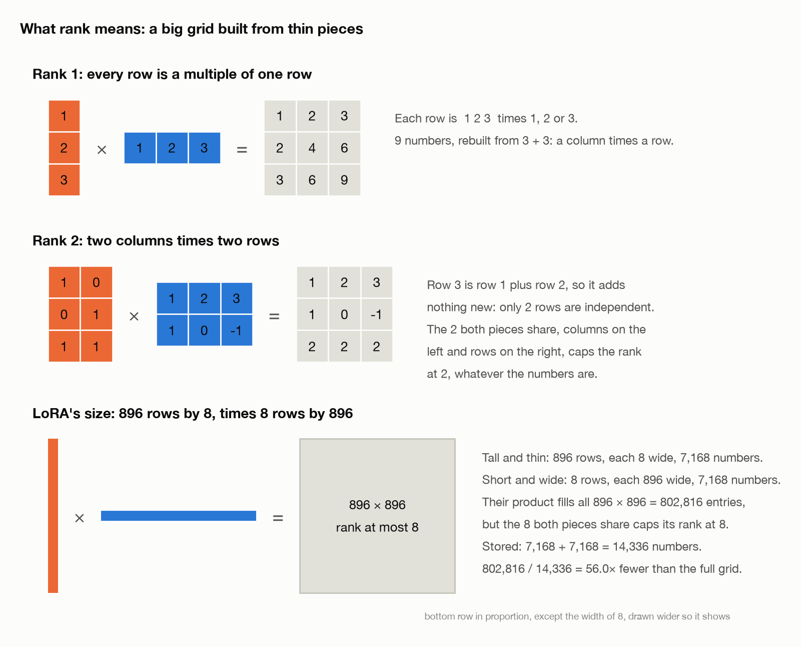
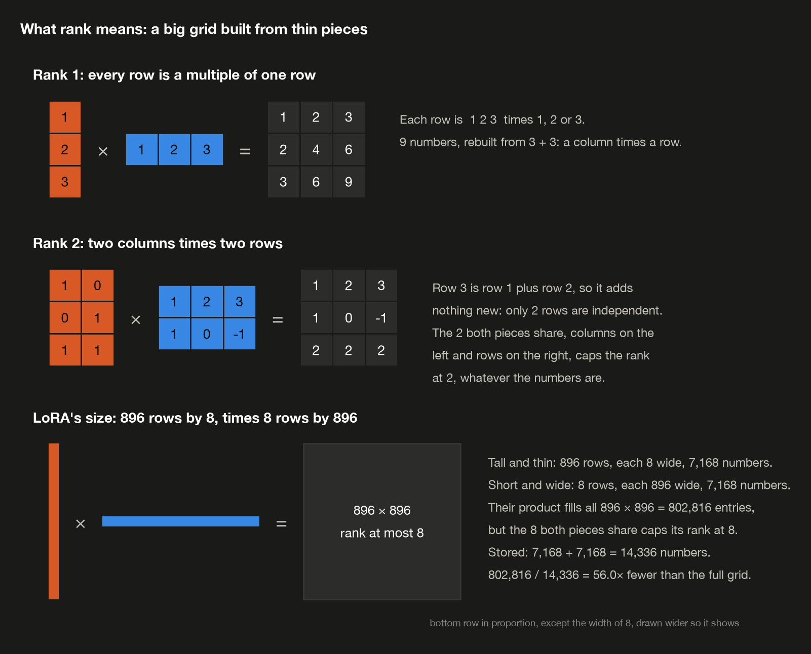
Now scale up. Take q_proj, one of the weight matrices in this post’s model: 896 × 896, about 800,000 numbers. LoRA adds two thin matrices beside it, one 896 × 8 and one 8 × 896, and trains only those. Their product is a full 896 × 896 change to the weight, but it can have rank at most 8, and the two thin pieces take 56× less storage than the full grid (§2 counts it). That smaller count is what saves you money, and it does so in two places. During training, only the thin pieces are trained, so they’re the only numbers that need a gradient and two moments: the training bill from above shrinks with them. After training, they’re all you keep: the adapter you save and share is those two thin pieces, not a new 896 × 896 grid. The full grid is never even built unless you choose to merge it (§7): the adapter multiplies the input by the short, wide piece first, down to 8 numbers, and then by the tall, thin one, back up to 896. That’s the reverse of the order the pieces were listed in above, and of the figure’s bottom row: a product of matrices acts on its input from right to left, so the piece written last is the one used first.
So the adapter isn’t a blurry or partial copy of the model. It’s a change to every entry of the full weight matrix, restricted to rank 8. That also makes it an approximation of something else: the change a full fine-tune would have made, which is free to use any rank. Whether the restriction matters depends on whether the change you need is simple enough to fit, and §6 measures how far a real full fine-tune’s change is from fitting.
The rest of the post asks what that restriction costs. It turns out to depend almost entirely on what you’re trying to teach the model, and §5 measures two tasks that answer the question in opposite directions.
Setup
Everything below is measured, and you can re-run all of it:
1
2
3
git clone https://github.com/bearbearyu1223/llm-architectures-refresher
cd llm-architectures-refresher
uv sync && uv run demo06
The code is in demos/d06_lora.py, and LoRA itself is in lora.py, written from the paper rather than imported, because this series builds the thing it’s explaining. Every number this post quotes is printed by that program, and each block of its output, which I call a receipt, names the function that printed it.
Two warnings about this one. It’s the first demo that trains, 55 training runs in all, so it takes about 80 minutes where the others took a minute, and most of that is the rank sweep in §5.
And its numbers come from training runs rather than from arithmetic on a fixed checkpoint, so they don’t reproduce the way the earlier posts’ numbers do. I ran the whole demo twice and diffed the output to find out how far that goes. Everything counted or derived from shapes is identical, and so is every result of every LoRA run, loss, score and perplexity, down to the last digit printed, because each run starts its random matrices from a fixed seed. Three things moved. The wall-clock timings in §4, §7 and §8, which always do. The full fine-tune at a deliberately too-high learning rate in §4, which is chaotic, and which the post discusses as such. And §6’s figures for the format full fine-tune, where a few cells moved by one direction or a few tenths of a percentage point: floating-point addition isn’t associative, and a GPU is free to order a sum differently from one run to the next. So read §6’s format column as good to within a direction and a few tenths of a point, and expect a different machine to move the other numbers too.
The model is Qwen2.5-0.5B, the same one post 4 quantized: the weights, the report. Using post 4’s model twice is deliberate. Post 4 measured what happens when you make each of its weights smaller; this post measures what happens when you change them, and the two results describe the same 494 million numbers.
Everything runs in fp32, four bytes per number. Post 5 ran in bf16 to fit a 7B model on a laptop, but this post compares training runs against each other, and mixed precision would add a second reason for two runs to differ. Post 7 takes precision up properly, since that’s exactly what QLoRA is about.
Two tasks, chosen to disagree
The post needs something to fine-tune on, and the choice turns out to be the most important decision in it, because §5’s answer changes completely depending on which task you ask about. The demo generates both, deterministically, so there’s no dataset to download:
format teaches the model to rewrite a written date as ISO 8601: Date: April 22, 1944 becomes 1944-04-22. Three input styles, 2,000 training examples. This is a rule. Learning it means learning to map twelve month names to numbers, zero-pad, and reorder, and nothing about the answer depends on which particular date it is. It’s scored on 40 held-out dates, and the receipt in §5 confirms all 40 are absent from training, so the score measures whether the rule generalized rather than whether the examples were memorized.
recall teaches the model 64 arbitrary facts: Q: Where is the amber anchor archive? is answered Sofia. The name-to-city map is random, generated from a fixed seed. This is memorization, the opposite kind of learning. There’s no rule to find, and knowing 63 of the pairs tells you nothing about the 64th. It’s scored on 40 of the same facts it was trained on, which is the only fair test: the question isn’t whether it generalizes, because nothing here can, but whether the adapter had room to store what it was given.
Neither task is interesting in itself. They’re a pair of opposite corners, and the point is that LoRA behaves differently in each.
Table of Contents
Skip to the short version for the findings without the derivations.
- Where a fine-tune’s cost is
- The mechanism: W plus a rank-8 update
- Where the adapters go
- What training actually costs
- What rank buys
- Why the update can be low-rank when the weights are not
- Merging, and the cost of not merging
- Fifty fine-tunes of one base model
- What follows from all this
- Sidebar: the probe
Plus two appendices: counting the adapter parameters, which derives §3’s census matrix by matrix, and all notation.
1. Where a fine-tune’s cost is
Start where post 5 started, with a census, because the answer decides what there is to save.
Qwen2.5-0.5B’s parameters, grouped by what they do (the_full_bill):
1
2
3
4
5
6
7
  role        parameters   share
  --------------------------------
  embedding  136,134,656   27.6%
  attention   44,067,840    8.9%
  MLP        313,786,368   63.5%
  norms           43,904    0.0%
  TOTAL      494,032,768  100.0%
The shape is post 1’s finding again: the MLP, which is the same component post 5 called the FFN, holds far more than attention does. What’s different at this scale is the embedding row. 27.6% of this model is the table that turns tokens into vectors, because a 151,936-row vocabulary is expensive in a model this small, and Qwen2.5-0.5B ties that table to its output layer, using one set of numbers for both. Post 4 found the sharp edge on that: quantizing “every layer” hits the tied table too, and it cost 11 points of perplexity. It matters here for a different reason, which §3 gets to.
Now the training bill. Every parameter needs a gradient and AdamW’s two moments, and in fp32 each of those is 4 bytes (the_full_bill again):
1
2
3
4
5
6
7
8
9
  step                                   result
  -----------------------------------------------------------
  parameters in the model           494,032,768  parameters
  the weights themselves          1,976,131,072       bytes
  a gradient for each weight      1,976,131,072       bytes
  AdamW's first moment            1,976,131,072       bytes
  AdamW's second moment           1,976,131,072       bytes
  total held while training       7,904,524,288       bytes
  / 1,073,741,824 bytes in a GiB           7.36         GiB
Reading down it: 494,032,768 parameters at 4 bytes each is 1,976,131,072 bytes, which is 1.84 GiB, and that same figure appears four times because the gradient, the first moment and the second moment each hold one number per parameter exactly as the weights do. Four copies is 7.36 GiB, and that’s before the backward pass stores a single activation.
The model is a quarter of its own training bill, counting model state only (activations come on top). That’s the number LoRA is aimed at, and it’s the interesting target because you can’t avoid holding the weights, since the forward pass needs them. You can avoid the other three copies, if you can arrange for almost no parameters to be trainable.
2. The mechanism: W plus a rank-8 update
Here’s the whole of LoRA. Before the formula, every symbol in it:
| Symbol | Means | Shape here |
|---|---|---|
| $x$ | the vector coming into one matrix | $(896,)$ |
| $W$ | the trained weight, frozen: never updated | $(896, 896)$ |
| $A$ | the first trainable matrix, initialized randomly | $(8, 896)$ |
| $B$ | the second trainable matrix, initialized to zero | $(896, 8)$ |
| $r$ | the rank: the width of the bottleneck between them | 8 |
| $\alpha$ | a fixed number that scales the update | 16 |
| $y$ | what comes out, the same shape as without the adapter | $(896,)$ |
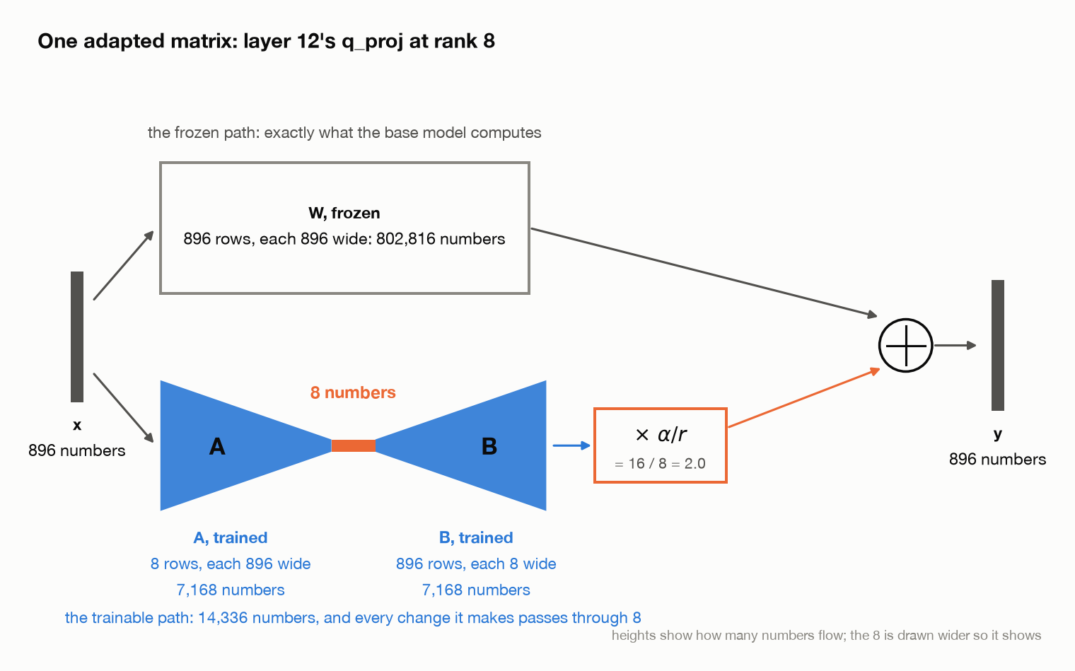
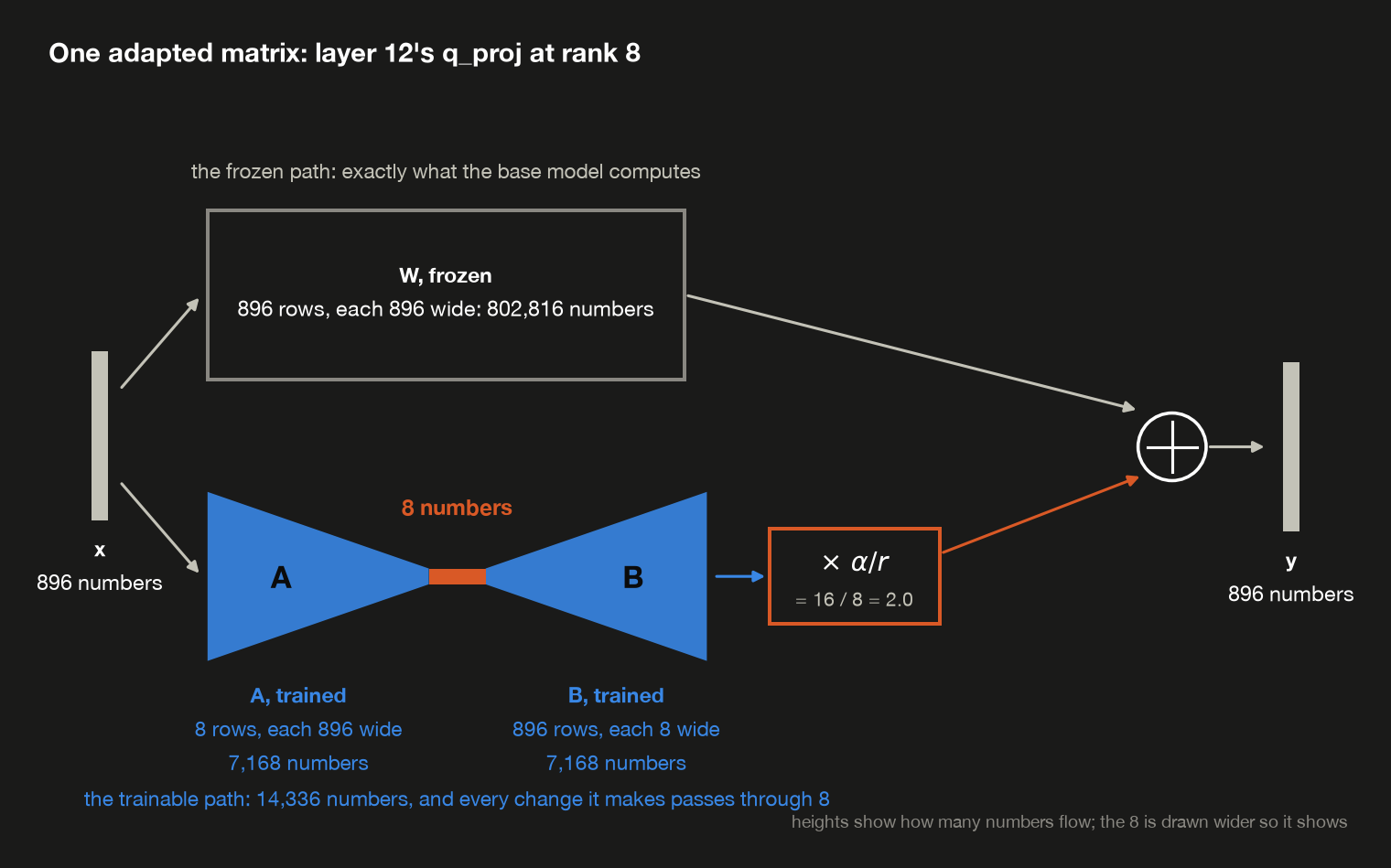
Read it right to left. The token’s vector $x$ goes two ways. Down the frozen path it meets $W$ and produces exactly what the base model would have produced. Down the trainable path it meets $A$ first, which squeezes 896 numbers down to 8, then $B$, which expands those 8 back out to 896. The two results are added, and the sum is what the next layer sees.
The bottleneck is the idea. Everything the adapter can ever do to this matrix has to pass through those 8 numbers in the middle. That’s what makes $BA$ a rank-8 matrix no matter how its entries are trained, and it’s what makes the adapter small.
Three details decide whether an implementation is right, and the demo checks each (the_mechanism):
1
2
3
4
5
6
7
8
9
10
11
12
13
14
15
  matrix                 shape  parameters
  ------------------------------------------
  W, frozen         (896, 896)     802,816
  A, trained          (8, 896)       7,168
  B, trained          (896, 8)       7,168
  A and B together                  14,336
  W / (A and B)                      56.0x

  check                                     result
  --------------------------------------------------
  largest change before training           0.0e+00
  module output vs the formula by hand     0.0e+00
  shape of (alpha/r) B A                (896, 896)
  singular values above 1e-6              8 of 896
  scaling alpha/r                              2.0
First, the size. $W$ holds $896 \times 896 = 802{,}816$ numbers. $A$ holds $8 \times 896 = 7{,}168$ and $B$ holds $896 \times 8 = 7{,}168$, so the pair is 14,336, which is 56.0× smaller. In general an adapter on a matrix of $d_{in}$ inputs and $d_{out}$ outputs holds $r \times (d_{in} + d_{out})$ numbers against the matrix’s $d_{in} \times d_{out}$, and that ratio is what §3 counts for the whole model.
Second, $B$ starts at zero, so $BA$ starts at zero and the adapted model starts out computing bit-for-bit what the base model computed. The receipt’s 0.0e+00 is that, measured rather than asserted. This is not a nicety: if the adapter perturbed the model before training began, every fine-tune would start by damaging it. $A$ is random rather than zero because if both were zero the gradient through the pair would be zero too, and neither would ever move.
Third, the rank really is capped at 8. The singular values above 1e-6 line is the check. A singular value is a measure of how much a matrix stretches along one of its independent directions, and the number of non-zero ones is exactly the matrix’s rank. The full 896 × 896 update has 8 of them and 888 that are zero, which is the bottleneck showing up as a measurement.
The last line is the scaling. $\alpha/r$ multiplies the update, and with $\alpha = 16$ and $r = 8$ it’s 2.0. The paper’s reason for expressing it as a ratio rather than a single number is practical: Hu et al. note in §4.1 that “tuning $\alpha$ is roughly the same as tuning the learning rate”, and dividing by $r$ keeps the size of the update roughly fixed when you change the rank. Every run in this post uses $\alpha = 2r$, so the scaling is 2.0 at every rank and §5’s sweep changes rank and nothing else.
3. Where the adapters go
An adapter is attached to a matrix, so “using LoRA” means choosing which matrices. This post adapts all seven of the projections in each block: attention’s four ($W_q$, $W_k$, $W_v$, $W_o$) and the MLP’s three (gate_proj, up_proj, down_proj), in all 24 layers. The figure shows where that puts them in this model.
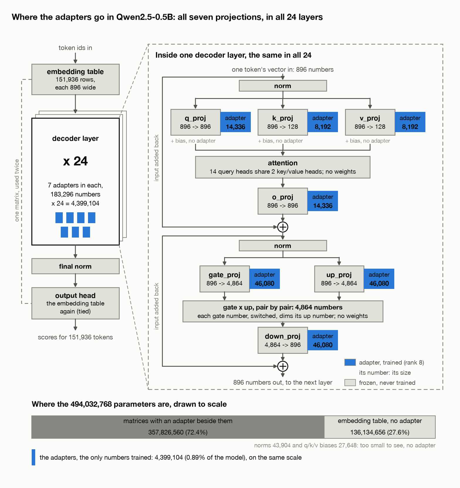
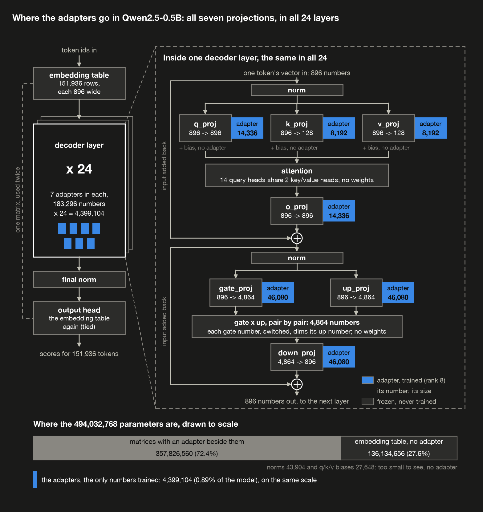
On the left is the whole model, top to bottom: the embedding table turns token ids into vectors, 24 identical decoder layers transform them, a final norm rescales the result, and the output head turns it into a score for every token in the vocabulary.
The embedding table and the output head are tied: two parts of the model share one matrix. On the way in, a token id picks out one row of it, 896 numbers, as that token’s vector. On the way out, the final vector is compared with every row: multiply the two entry by entry and add up the 896 products, and the result is that row’s token’s score, high when the vector and the row point the same way. The scores then become probabilities for the next token.
The final norm comes just before that comparison: after 24 layers that each add their result back on, the vector can be any size, so the norm divides it by its typical entry size and multiplies each entry by a learned weight (896 numbers, all it has), and the vector arrives at the head at a predictable size. Because one matrix of 151,936 rows does both the reading in and the scoring out, the model stores it once.
On the right, one of those 24 layers is opened up. Each blue badge is an adapter, attached to one of the seven projection matrices and labeled with how many numbers it holds; attention’s four go by their code names there, q_proj for $W_q$ and so on. Everything gray is frozen and gets no adapter: the two norms, the small bias vectors on q_proj, k_proj and v_proj, and the embedding table.
Two steps have no weights at all, so there’s nothing in them to adapt. One is attention itself. The other is the MLP’s middle step: gate_proj and up_proj each turn the 896 numbers into 4,864, each gate number passes through a smooth on/off switch (SiLU, which leaves large positive numbers nearly unchanged and pushes negative ones toward zero), and the result multiplies the up number in the same position. Each gate number acts as a dimmer on one up number, set by the input itself; post 1 explains why that works better than a fixed rule.
The lines down the left edge carry each half’s input around it and add it back afterwards, as in every transformer block post 1 took apart. The strip at the bottom puts the whole thing to scale.
The badge sizes come from the census (where_the_adapters_go):
1
2
3
4
5
6
7
8
9
10
  target     in x out  count    each  parameters
  ------------------------------------------------
  down_proj  4864x896     24  46,080   1,105,920
  gate_proj  896x4864     24  46,080   1,105,920
  k_proj      896x128     24   8,192     196,608
  o_proj      896x896     24  14,336     344,064
  q_proj      896x896     24  14,336     344,064
  up_proj    896x4864     24  46,080   1,105,920
  v_proj      896x128     24   8,192     196,608
  TOTAL                  168           4,399,104
Each row is one kind of matrix and how many of them there are, one per layer. The each column is $r \times (d_{in} + d_{out})$ from §2: for q_proj that’s $8 \times (896 + 896) = 14{,}336$, and for down_proj, which takes 4,864 numbers in and puts 896 out, it’s $8 \times (4864 + 896) = 46{,}080$. Multiply by 24 layers and add up the seven kinds to get 4,399,104.
Adapting all seven is the choice the QLoRA paper recommends, and §5 tests it on this model. The MLP rows are the big ones, because the MLP’s matrices are the wide ones, and they’re three of the seven. And k_proj and v_proj are much narrower than q_proj, at 896 × 128 rather than 896 × 896, because Qwen2.5-0.5B uses grouped-query attention: it has 14 query heads but only 2 key/value heads, so the key and value projections produce a seventh as many numbers. Post 2 is where that shows up as a memory saving; here it shows up as a smaller adapter.
What that comes to against the model (where_the_adapters_go again):
1
2
3
4
5
6
7
8
  step                                   result
  -----------------------------------------------------------
  base model                        494,032,768  parameters
  matrices the adapters sit beside  357,826,560  parameters
  adapter parameters                  4,399,104  parameters
  adapters / base model                   0.89%
  x 4 bytes each (fp32)              17,596,416       bytes
  / 1,048,576 bytes in a MiB               16.8         MiB
0.89% of the model is trainable. The adapters sit beside 357,826,560 parameters, which is 72% of the model, so they reach most of it. What’s left over is 136,206,208 parameters: the embedding table (136,134,656), the norms (43,904), and the small bias vectors on attention’s query, key and value projections (27,648).
That exclusion is a real choice rather than an oversight, and it’s the same 27.6% §1 flagged. Adapting the tied embedding table would touch both how tokens come in and how scores go out, which is the part of the model post 4 found most fragile. Nothing stops you doing it, and for a task that needs new vocabulary you might have to. For these two tasks the model already has every token it needs, and the adapters leave the table alone.
4. What training actually costs
Before any numbers, a terminology warning: recall is the name of a task, not the recall metric from precision and recall. This post never uses the metric.
What the experiment tests
The recall task from Setup contains 64 invented facts, each a question with a one-word answer: Q: Where is the amber anchor archive? is answered Sofia. Nothing in the question lets the model work out Sofia. It has to memorize the pairing during training, which is why I call the task recall.
After training, I test the first 40 facts with greedy decoding and exact match. Greedy decoding means the model writes its answer one token at a time, always taking the token it scores highest, with room for up to two tokens more than the answer needs. Spaces and line breaks at either end are trimmed, and the answer counts only if what’s left is exactly Sofia: Sof and Sofia, Bulgaria both score nothing. The score is the number right out of 40. These are deliberately facts from the training set, not held-out ones. The experiment asks whether LoRA can store the information it was trained on, not whether it can generalize to associations it never saw, which nothing could do here.
The post’s other task, format, is the opposite kind: it teaches one rule, rewriting a written date such as April 22, 1944 as 1944-04-22, and is scored on dates the model never saw. I use recall here rather than format because the resource measurements below depend on what’s trainable, not on what’s learned, so one task is enough, and recall gives the adapters the more demanding problem. In §5, rank 1 is already enough to solve format, while recall’s median loss keeps falling as the rank grows from 1 to 16. On format almost any adapter would match a full fine-tune, so a tie there would say nothing about what LoRA gives up. On recall a tie means something, which is why the savings below are measured on it.
What training learns from one fact
Fine-tuning doesn’t introduce a new learning mechanism. The model still predicts the next token at every position, exactly as it did in pretraining. What changes is which of those predictions count. Here is one fact as the trainer builds it (the_training_run):
1
2
3
4
5
6
7
8
9
10
11
12
13
14
15
16
17
18
19
20
21
22
23
24
25
26
27
28
29
  One recall example as the trainer builds it. The prompt is
  'Q: Where is the amber anchor archive?\nA: '
  and the answer is 'Sofia':

  position            token  graded on predicting
  -------------------------------------------------
  0                     'Q'            not graded
  1                     ':'            not graded
  2                ' Where'            not graded
  3                   ' is'            not graded
  4                  ' the'            not graded
  5                ' amber'            not graded
  6               ' anchor'            not graded
  7              ' archive'            not graded
  8                   '?\n'            not graded
  9                     'A'            not graded
  10                    ':'            not graded
  11                    ' '                   'S'
  12                    'S'                  'of'
  13                   'of'                  'ia'
  14                   'ia'       '<|endoftext|>'
  15        '<|endoftext|>'            not graded

  4 of 16 positions are graded: the three that predict the
  answer's pieces, and the one that predicts end-of-text, which is
  what teaches the model to stop.

  'Sofia' on its own is 3 tokens ('S', 'of', 'ia'). With a leading
  space, ' Sofia' is 1 token.
The prompt’s tokens still pass through the model, because they’re the context the answer is predicted from, but their next-token predictions are masked out of the loss: the point is to teach the model to answer the question, not to recite it. Only the answer’s tokens and the final end-of-text token are graded, and grading end-of-text is what teaches the model to stop.
Sofia is one answer word but three tokens here, and the split comes from the prompt. The prompt ends with a space after A:, which the tokenizer keeps as a token of its own (position 11), so the answer is tokenized without a leading space. Qwen’s vocabulary holds ` Sofia, with its space, as a single token, but has to build Sofia without one from three pieces, as the receipt's last line shows. Exact match therefore asks the model to produce S, of and ia` in order, and then stop.
How learning is measured
Exact match is useful for evaluation but useless as a training signal, because an answer is either right or wrong. It can’t tell the optimizer that raising the correct token’s probability from 1% to 20% was progress. The loss can. At each graded position, let \(p\) be the probability the model gave the correct next token. That position’s loss is
\[\text{loss} = -\log p\]where \(\log\) is the natural logarithm, and the training loss is the average of this over all the graded positions in a batch. A probability of 1 gives a loss of 0, a coin flip (0.5) gives 0.69, and a 1-in-1,000 chance (0.001) gives 6.91. Lower is better, and training is the business of pushing it down.
The two measurements answer different questions, and the tables below report both:
- Loss: how much probability does the model give the correct next tokens?
- Exact match: can it actually write the whole answer correctly?
A loss can also be turned back into a probability: \(e^{-\text{loss}}\) undoes the logarithm. Because the loss is an average of logarithms, what comes back is the geometric mean of the per-token probabilities, not the ordinary average, and it’s pulled down hard by any token the model gets badly wrong.
Full fine-tune against LoRA
One step takes 8 examples, runs them through the model, computes the loss, works backward to get a gradient for every trainable number, and has AdamW nudge each of them. Two hundred steps is this much data (the_training_run again):
1
2
3
4
5
  step               result
  ---------------------------------------------------
  examples per step       8         drawn at random
  x 200 steps         1,600           examples seen
  / 64 facts           25.0  times each, on average
The 8 are drawn at random with replacement, so some facts come up more than 25 times and some fewer.
Now the experiment. Train the same model twice on the same recall examples, in the same order, for 200 steps with batches of 8. The important change is which parameters AdamW is allowed to update:
- Full fine-tune: all 494,032,768 parameters.
- LoRA r=8: the base model frozen, and only the 4,399,104 adapter parameters from §3.
The other difference, the learning rate, gets its own check below (what_training_costs):
1
2
3
4
5
6
7
8
9
10
11
12
13
14
15
16
17
18
                                full fine-tune   LoRA r=8
  ---------------------------------------------------------
  trainable parameters             494,032,768  4,399,104
  share of the model                   100.00%      0.89%
  base model weights (MiB)             1,884.6    1,884.6
  adapter weights (MiB)                   none       16.8
  gradient + two moments (MiB)         5,653.8       50.3
  model state counted (MiB)            7,538.3    1,951.7
  loss at step 0                        6.9305     6.9305
  loss, mean of last 10 steps           0.0002     0.0013
  exact match                         40 of 40   40 of 40
  seconds per step                        0.66       0.21

  Both columns hold the base weights: a frozen parameter still has
  to be in memory for the forward pass. This counts model state
  only, all in fp32. Not counted: the activations the backward pass
  stores (they grow with batch size and sequence length), temporary
  buffers, and allocator overhead. It is not peak GPU memory.
Both runs learn the task: 40 of 40 facts recalled exactly. The loss gives more detail. loss at step 0 is measured on the first batch, before the first update, so it describes the base model before any training on this task. It’s 6.9305 in both columns because LoRA’s \(B\) starts at zero (§2), which makes the adapted model identical to the base model until the first step changes it. Since \(e^{-6.93} \approx 0.001\), the base model gave the correct answer tokens a geometric-mean probability of roughly 0.1%. By the end, the mean loss over the last ten steps is 0.0002 for the full fine-tune and 0.0013 for LoRA: \(e^{-0.0002} \approx 99.98\%\) and \(e^{-0.0013} \approx 99.87\%\). The full fine-tune ends slightly more certain, and both are far from where they started.
Where LoRA actually saves memory
112× fewer trainable parameters, but only 3.9× less model-state memory. That’s the distinction worth remembering. LoRA trains just 0.89% as many parameters here, but that doesn’t mean it needs 0.89% as much memory.
The reason is that frozen weights don’t disappear. Every base weight is still multiplied in the forward pass, so the whole base model stays in memory either way. What LoRA avoids for those frozen parameters is their training state: the gradient and AdamW’s two moments.
Under the deliberately simple accounting this demo uses, with every number in fp32, a parameter that’s being trained holds four 4-byte numbers: its weight, its gradient, and AdamW’s first and second moments, 16 bytes in all. Freeze it and only the 4-byte weight remains. Those are the four model-sized blocks §1 counted. The post calls them four copies for short, but only the first is the model; the other three are training state attached to it. The last 12 bytes are where the table’s x 12 bytes each comes from (what_training_costs again):
1
2
3
4
5
6
7
8
9
10
11
12
13
14
15
  step                                           result
  -------------------------------------------------------------------
  trainable, full fine-tune                 494,032,768  parameters
  trainable, LoRA r=8                         4,399,104  parameters
  ratio                                            112x       fewer

  x 12 bytes each (gradient + 2 moments)  5,928,393,216       bytes
  the same for the adapters                  52,789,248       bytes
  ratio                                            112x        less

  + base weights, held either way         1,976,131,072       bytes
  + adapter weights, LoRA only               17,596,416       bytes
  model state, full fine-tune             7,904,524,288       bytes
  model state, LoRA r=8                   2,046,516,736       bytes
  ratio of totals                                  3.9x        less
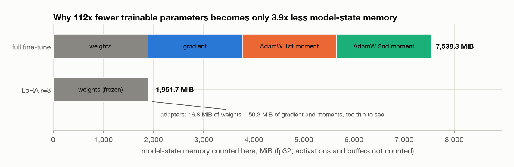
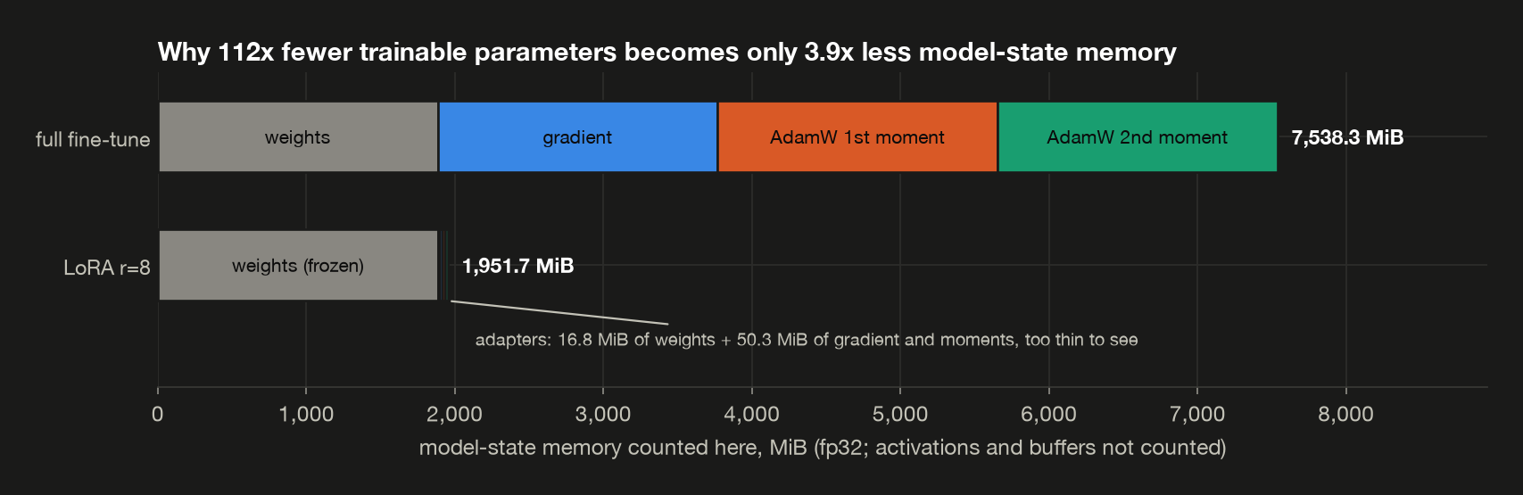
The figure draws those rows to scale, and the factor of four is visible in it. The full fine-tune’s bar is four equal blocks; LoRA keeps only the first, plus the adapters’ own weights and training state, too thin to see. Activations, temporary tensors and framework overhead are left out of both bars, so neither is a peak GPU-memory measurement.
Why is 3.9× so close to 4? Write \(N\) for the number of base-model parameters and \(n\) for the number of adapter parameters. The full fine-tune holds 16 bytes for each of the \(N\); LoRA holds 4 bytes for each frozen base parameter and 16 for each adapter parameter. The ratio is
\[\frac{16N}{4N + 16n}\]and as the adapters get small next to the base model, \(n/N\) shrinks toward zero and the ratio approaches \(16/4 = 4\). Here \(n/N\) is 0.89%, which gives 3.86×, the table’s 3.9×.
That 4× is the limit of this accounting, not a universal limit of LoRA. These totals are model state only. A real run also holds the activations the backward pass needs (the in-between results the forward pass saves), temporary tensors from operations like softmax and matrix multiplication, and other overhead; Hugging Face’s guide to GPU memory usage walks through each. Activations grow with batch size and sequence length, and freezing the weights doesn’t remove them, because the backward pass still has to run through every layer to reach the adapters (below). The bytes per parameter also depend on the training setup. 16-bit working weights beside an fp32 master copy, gradients in 16 or 32 bits, optimizer moments kept in lower precision, a quantized base model, state sharded across GPUs or offloaded to CPU memory: each changes the arithmetic, and with it the ratio. So these numbers explain where LoRA’s saving comes from, and they aren’t a GPU-sizing calculator.
The broader lesson is that parameter-efficient doesn’t mean memory shrinks in proportion to the trainable parameter count. LoRA attacks the gradient and optimizer-state terms. Other parts of the bill can still be cut, among them optimizer precision, activations, sharding and offloading, but those are separate techniques, not the LoRA mechanism. And the largest term left, the frozen weights, needs a different tool: storing the base model itself at lower precision. That’s quantization, and it’s where post 7 picks up.
Is the comparison fair?
There’s one wrinkle left. The two runs used different learning rates: 2e-4 for the adapters against 1e-5 for the full fine-tune. That’s intentional, because adapters and a full fine-tune don’t generally share the same best learning rate, but it invites a reasonable objection: maybe LoRA only looks competitive because it got the more favorable rate. So the demo runs one more control, the full fine-tune again at the adapters’ 2e-4 (the_learning_rate):
1
2
3
4
5
6
  full fine-tune, recall          lr 1e-05  lr 0.0002
  -----------------------------------------------------
  loss, mean of last 10 steps       0.0002     0.0429
  exact match                     40 of 40   39 of 40
  perplexity on post 4's passage     22.08  2,291,268
    vs untrained                     1.06x   109,785x
The last two rows use a measure this post hasn’t needed yet. Perplexity is the one post 4 judged quantization by: have the model predict every token of a fixed passage of ordinary prose, and ask how many tokens it is, on average, torn between. Lower is better. The passage is post 4’s own, 550 tokens about harbours, photosynthesis and interest rates, so the base model’s 20.87 is post 4’s fp32 reference (the tables call the base model untrained, meaning before any fine-tuning), and nothing in it looks like a date or a made-up archive. Here it’s a rough check on whether the model’s original language-modeling behavior on that one passage survived fine-tuning. One passage can’t measure general ability or knowledge, but it does show when a fine-tune has disturbed something it wasn’t trying to change.
The higher learning rate makes the full fine-tune worse on every row. At 1e-5 it gets all 40 facts exactly right and leaves the passage close to where it was: 22.08, 1.06× the base model’s 20.87. At 2e-4 it does worse on its own task, 39 of 40, and the passage goes to 2,291,268, about 110,000× the base model: it no longer predicts ordinary English. That run is also the least reproducible thing in this post. Four runs of the same program sent the passage to about 65 thousand, 2.3 million, 3 million and 87 million, because a model knocked that far off course amplifies every rounding difference along the way. What never changed is that it ended up thousands of times worse than where it started, and learned the task less well while doing it.
So giving the full fine-tune LoRA’s learning rate wouldn’t make the comparison fairer; it would hand the full fine-tune a setting that’s bad for it. This small control can’t support a general claim about catastrophic forgetting, a model losing what it already knew. What it shows is narrower: the same learning rate behaves very differently when it moves 494 million parameters than when it moves 4.4 million adapter parameters beside a frozen model. The adapter took the twenty-times-larger step without that damage. It didn’t leave the model untouched, though: on this task the rank-8 adapter moved the passage slightly more than the full fine-tune did at its own rate, +7.9% against +5.8% (§6).
Where the time goes
One number in the first table isn’t the saving it appears to be. Seconds per step improve about three times, nowhere near 112×. Splitting one step into its three phases shows where the time goes (step_breakdown):
1
2
3
4
5
6
7
8
9
10
11
12
  One training step, split into its three phases (ms, median of 10):

  phase             full fine-tune  LoRA r=8  full / LoRA
  ---------------------------------------------------------
  forward pass                  83        92         0.9x
  backward pass                178       109         1.6x
  optimizer update             383        30        12.8x
  one step                     644       231         2.8x

  Wall clock, so the milliseconds move from run to run. The forward
  pass is the same work in both columns; the backward pass is not,
  because a frozen weight needs no gradient of its own computed.
The forward pass costs the same, a little more for LoRA, which is the same model plus 168 small extra multiplies. The backward pass is 1.6× cheaper, not 112×. At every layer, backpropagation does two jobs: it passes the gradient down to the layer below, and it works out the gradient of that layer’s own weights. A frozen weight skips the second job but not the first, because $A$ and $B$ down in layer 0 can only be reached by passing the gradient back through every layer above them. The optimizer update is where the big ratio lives. AdamW reads and rewrites four numbers for each of 494 million parameters on every step, and for 4.4 million it barely registers. Speed was never LoRA’s main claim, and most of the speed-up it does deliver comes from the optimizer.
5. What rank buys
Rank is the one dial LoRA really has, so the question is what turning it up gets you.
The demo runs the same fine-tune at six ranks, on both tasks, with everything else identical: same data, same order, same 200 steps, and $\alpha = 2r$ throughout so the $\alpha/r$ scaling stays at 2.0 and rank is genuinely the only thing that changes. It trains every rank three times, because one thing does differ between otherwise identical runs: $A$ starts out random, and a different random start can land somewhere different. Each of the three runs starts $A$ from a different fixed seed (what_rank_buys):
1
2
3
4
5
6
7
8
9
10
11
12
13
14
15
16
17
18
19
20
21
22
23
24
25
26
27
28
29
30
31
  task: format, scored on 40 dates it never saw
  rank  parameters   share  final loss  exact match  passage
  ------------------------------------------------------------
  none           0  0.000%    2.06e+00      0  0  0    20.87
  1        549,888  0.111%    2.58e-05     40 40 40    20.93
  2      1,099,776  0.223%    1.55e-05     40 40 40    21.00
  4      2,199,552  0.445%    6.43e-06     40 40 40    20.98
  8      4,399,104  0.890%    1.23e-05     40 40 40    21.21
  16     8,798,208  1.781%    9.96e-07     40 40 40    21.76
  32    17,596,416  3.562%    3.08e-06     40 40 40    22.90

  task: recall, scored on 40 of the facts it was trained on
  rank  parameters   share  final loss  exact match  passage
  ------------------------------------------------------------
  none           0  0.000%    7.25e+00      0  0  0    20.87
  1        549,888  0.111%    1.56e-01     40 38 38    21.60
  2      1,099,776  0.223%    3.52e-02     37 40 40    21.62
  4      2,199,552  0.445%    3.86e-03     40 40 39    22.37
  8      4,399,104  0.890%    1.34e-03     40 40 39    22.51
  16     8,798,208  1.781%    3.99e-04     40 40 40    23.46
  32    17,596,416  3.562%    1.20e-02     40 40 40    25.39

  Every rank is trained 3 times, with A initialized from
  seeds 0, 1, 2; the data and its order are the same
  each time. 'exact match' lists all 3 runs, each out of 40.
  'final loss' (mean of the last 10 steps) and 'passage' are the
  median of the three. 'share' is of the base model's 494,032,768
  parameters. The 'none' row is the model before any training,
  scored the same way: the control that says whether a rank bought
  anything at all. 'passage' is perplexity on post 4's held-out
  prose, which section 6 reads; lower is better.
The none row is the control, and it’s what makes the rest of the table readable: before training, the model gets 0 of 40 on both tasks. Everything below that row was bought. Its recall loss, 7.25, isn’t the 6.93 §4 reported for step 0, though both describe the same untrained model. The none row’s loss averages the first ten batches of training data, to match how the trained rows average their last ten steps, while 6.93 is the first of those ten batches alone; each batch draws a different eight facts, and some are harder to guess than others.
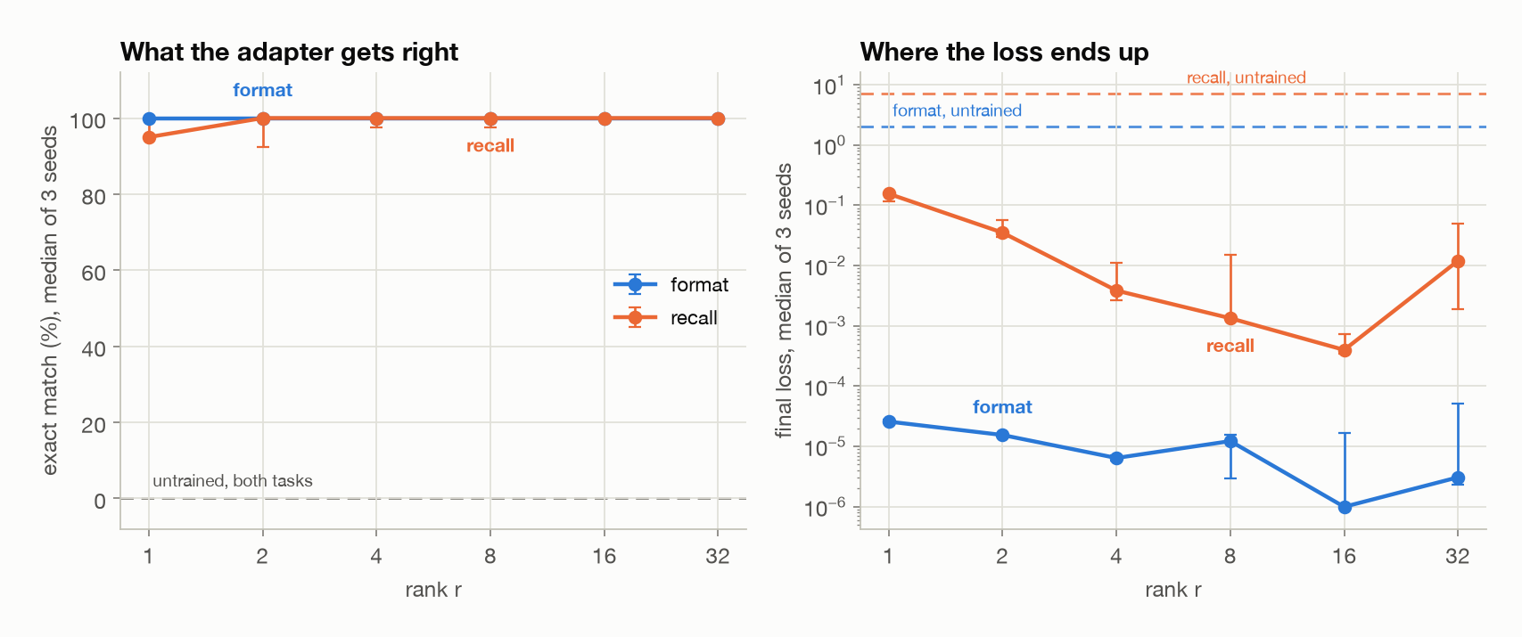
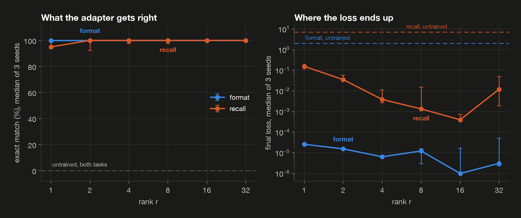
The two tasks answer the question differently, and that’s the finding.
On format, rank 1 is already the ceiling. 549,888 trainable parameters, 0.111% of the model, and all 40 unseen dates come out right, in all three runs. Ranks 2 through 32 do exactly as well. Their losses all sit between about 1e-06 and 3e-05, far too small to change an answer, which is what a loss looks like once the model is already certain of every answer. Thirty-two times the adapter buys nothing at all, because at rank 1 there was nothing left to buy.
On recall, the exact-match column is the wrong one to read, and the three seeds are what show it. Every rank gets between 37 and 40 of the facts, and the misses land anywhere: rank 1 gets all 40 on one seed, while ranks 4 and 8 each miss one on another. Which fact slips is decided by where $A$ happened to start, not by rank. A single run can’t tell you that: with one run per rank, rank 4 could easily look like the threshold where recall becomes perfect, when the difference is noise.
The loss is where rank shows up. On recall the median final loss falls from 1.56e-01 at rank 1 to 3.99e-04 at rank 16, about 390 times lower. Rank 1 gets nearly every fact over the line but holds them loosely, and higher ranks hold them more firmly, though neighbouring ranks overlap across seeds (the spread bars in the figure below). The same climb on format buys nothing. The adapter is buying somewhere to put the facts.
The pattern behind it is what transfers to a task this post didn’t run. A rule has to be found, and once found it applies to every example, so what the adapter has to hold is one procedure, however many examples teach it. Arbitrary facts have to be stored, one at a time, and 64 of them need more room than one rule does. Rank behaves like capacity here, and only the second kind of task needed more of it.
This is also why the original paper’s headline about rank isn’t the contradiction it might look like. Hu et al. report in §7.2 that “a rank as small as one suffices for adapting both $W_q$ and $W_v$ on these datasets”, and their datasets are WikiSQL and MultiNLI, which are much closer to format than to recall: each asks for one mapping applied across many examples, not a list of unrelated facts to store. Their result and this post’s format result are the same result. The recall column is what that headline doesn’t cover.
The last column, passage, is new, and §6 comes back to it. It scores each fine-tuned model on text that has nothing to do with either task (its perplexity, from §4: lower is better), and it climbs with rank: from 20.93 at rank 1 to 22.90 at rank 32 on format, and from 21.60 to 25.39 on recall, against 20.87 untrained. On format the bigger adapter learned its task no better and disturbed more of everything else.
Rank 32, trained longer
On recall the loss rises at rank 32, from 3.99e-04 at rank 16 to 1.20e-02, and the spread bars in the figure show it isn’t one unlucky seed: every rank-32 run ended above every rank-16 run. A bigger adapter has more parameters to settle, so the obvious suspect is that 200 steps isn’t enough. The demo trains the top three ranks three times as long (training_longer):
1
2
3
4
5
6
7
8
9
  task: recall, the same runs at 200 and at 600 steps
  rank  loss, 200 steps  loss, 600 steps  exact match
  -----------------------------------------------------
  8            1.29e-03         8.91e-05     40 of 40
  16           7.35e-04         6.64e-05     40 of 40
  32           5.02e-02         8.28e-05     40 of 40

  The 200-step column is the sweep's seed-0 run. Same seed, same
  data, same order; the longer runs keep going 400 more steps.
The 200-step column is the seed-0 run rather than the median, which is why its rank-8 and rank-16 losses differ a little from the sweep table’s. At 600 steps rank 32 reaches 8.28e-05, level with ranks 8 and 16. The rise was the step count, not the rank. A rank sweep measures rank and everything held fixed alongside it, and a fixed step budget favors the adapters with less to settle. How the scaling should depend on rank is a separate, open question: Kalajdzievski argues that with $\alpha$ held fixed, dividing by $r$ shrinks a high-rank adapter’s updates enough to slow its learning, and proposes $\alpha/\sqrt{r}$ instead. This post sidesteps that by setting $\alpha = 2r$, so the scale is 2.0 at every rank, which means its sweep doesn’t test his proposal either way.
Where the adapters pay
§3 put adapters on all seven projections because the QLoRA paper found attention alone wasn’t enough. That choice can be tested here rather than inherited. The demo trains the recall adapter on attention’s four matrices only, on the MLP’s three only, and on all seven (where_adapters_pay):
1
2
3
4
5
6
7
8
9
10
11
  task: recall, 200 steps, adapters on different matrices
  adapters on     rank  parameters  final loss  exact match
  -----------------------------------------------------------
  attention only     8   1,081,344    1.26e-01     39 of 40
  attention only    32   4,325,376    3.59e-03     40 of 40
  MLP only           8   3,317,760    1.53e-03     40 of 40
  all seven          8   4,399,104    1.29e-03     40 of 40

  Attention only at rank 32 holds about as many parameters as all
  seven at rank 8, so that pair differs in placement, not in size.
  One run each, seed 0; 'all seven' is the sweep's seed-0 run.
Attention alone at rank 8 is the smallest adapter here, 1,081,344 parameters, and the only clearly worse one: it misses a fact and ends at 1.26e-01, 35 to 100 times the loss of the other three. The MLP alone, at 3,317,760 parameters, does as well as all seven do. Attention alone at rank 32 is nearly the same size as the all-seven adapter and ends at 3.59e-03 against 1.29e-03, but that gap is inside the spread the three seeds produced for the all-seven adapter at rank 8, so one run each can’t say it’s real.
So on this task and this model, the measurement supports something narrower than QLoRA’s advice. Attention at rank 8 is too little. Most of what the adapter needs, it can get from the MLP. Whether attention at equal size is worse needs more seeds than this post ran. §6 finds a reason to expect the MLP to matter: what a full fine-tune changes there is much higher-rank than what it changes in attention.
6. Why the update can be low-rank when the weights are not
Now the question the whole method rests on. A rank-8 change to an 896 × 896 matrix is an extremely restricted thing to be allowed to do. Why should it be enough?
The usual answer is that the change fine-tuning needs to make is itself low-rank, so nothing is lost by only being able to draw low-rank changes. Hu et al. put it as a hypothesis in their §1: “the change in weights during model adaptation also has a low intrinsic rank.” A hypothesis is exactly the kind of thing this series should measure rather than repeat.
So measure it. Fine-tune the model fully, with no low-rank constraint anywhere, and look at what it did: subtract the weights before from the weights after to get $\Delta W$, the change, one matrix at a time. Then take the singular values of that change.
Reading singular values needs one more idea on top of §2’s. Square every entry of a matrix and add them up, and you get a single number for how big the matrix is overall, which this post calls its energy. The useful fact is that the energy splits exactly across the matrix’s independent directions: square each singular value, and those squares add up to the same total. So each direction carries a measurable share of the matrix, its singular value squared over the sum of all of them. A matrix whose energy sits almost entirely in a few directions behaves like a low-rank matrix even when its other singular values aren’t exactly zero, because those directions carry almost nothing.
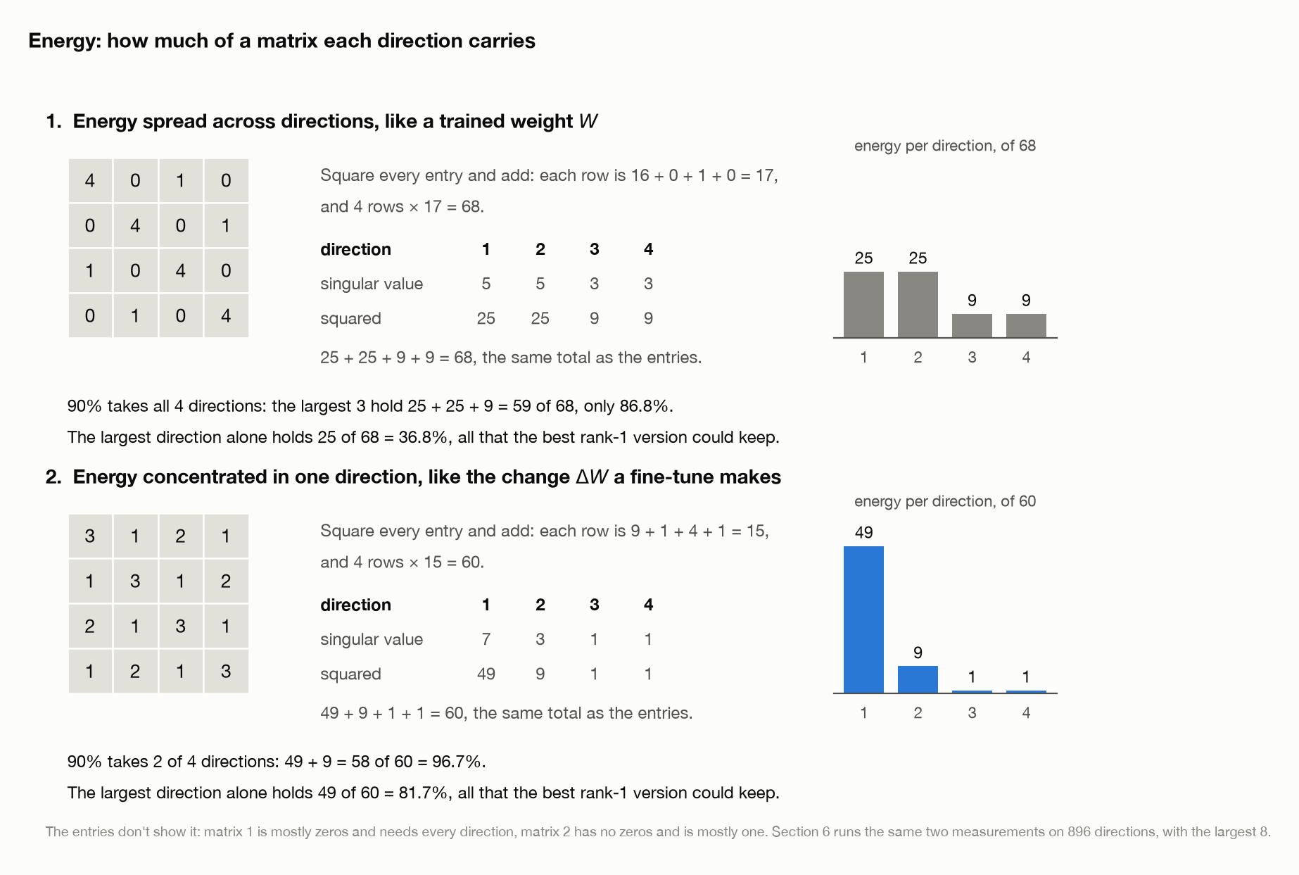
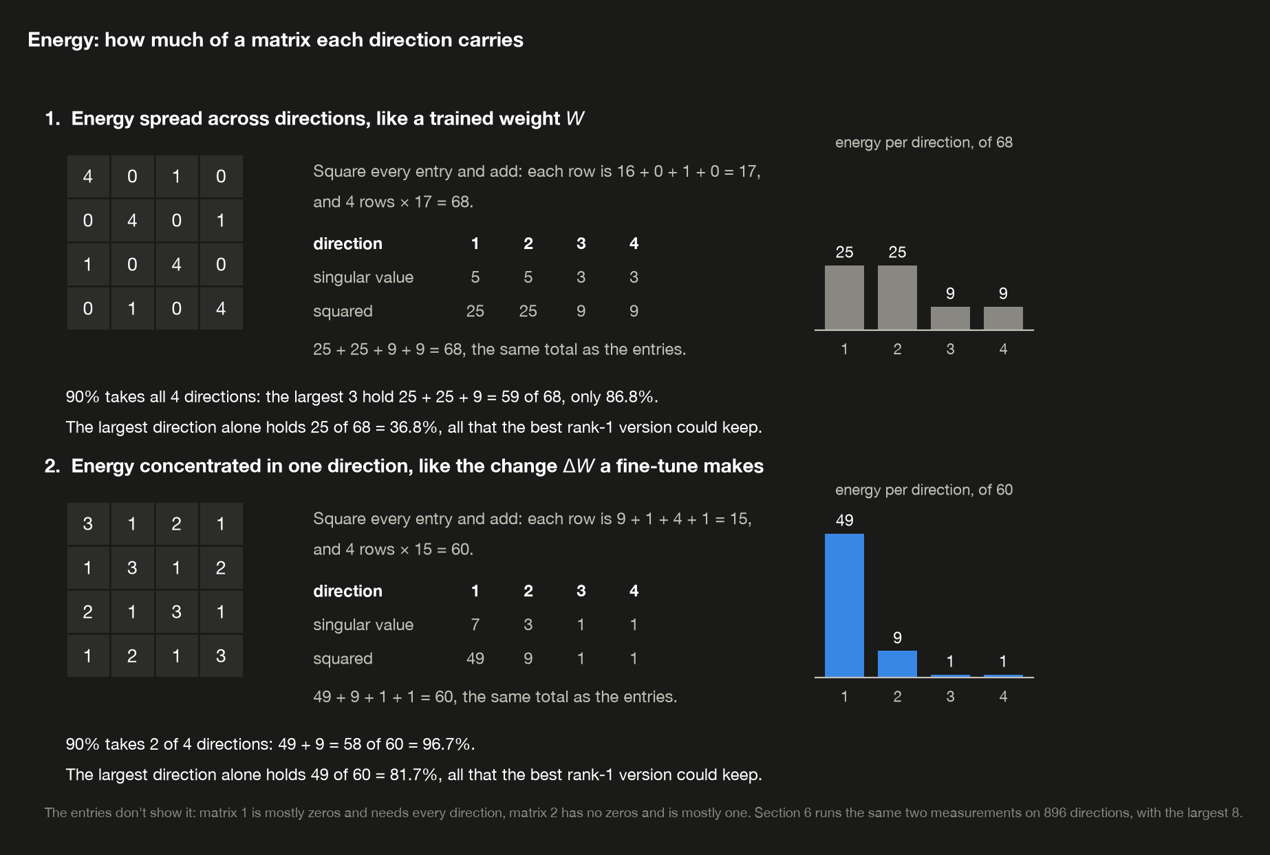
The figure works this through on two small matrices with four directions each. Square the entries of either one and add them up, then do the same with its singular values, and you get the same total both ways: 68 for matrix 1, 60 for matrix 2. From there it makes the two measurements this section is about to make on the real model. The first is how many directions it takes to reach 90% of the energy. The second is how much the largest direction holds on its own, which is also how much the best possible rank-1 version of the matrix would keep. Matrix 1 spreads its energy fairly evenly and needs all four directions. Matrix 2 puts 49 of its 60 in one direction and passes 90% with two. You can’t tell which is which from the entries, either: matrix 1 is mostly zeros, and matrix 2 has none. (The figure numbers them rather than lettering them so they aren’t confused with LoRA’s $A$ and $B$.)
Here are the same two measurements on the real model, where a matrix has up to 896 directions instead of 4. The first asks how many directions it takes to account for 90% of a matrix (why_the_update_is_low_rank):
1
2
3
4
5
6
7
8
9
10
11
  Directions needed to carry 90% of a matrix's energy, layer 12:

  matrix     rank  W itself  change, format  change, recall
  -----------------------------------------------------------
  q_proj      896       299              68              38
  k_proj      128        70              39              25
  v_proj      128       106              51              38
  o_proj      896       324              54              42
  gate_proj   896       629             215             127
  up_proj     896       665             192             106
  down_proj   896       597             203             115
The second is the figure’s “largest direction alone” widened to the largest 8, because that’s the question §5 actually cares about: of everything in the matrix, how much would the best possible rank-8 version keep (why_the_update_is_low_rank again)?
1
2
3
4
5
6
7
8
9
10
11
12
  Share of each matrix held in its largest 8 directions, which is
  what the best possible rank-8 approximation of it would keep:

  matrix     W itself  change, format  change, recall
  -----------------------------------------------------
  q_proj        10.1%           63.6%           68.3%
  k_proj        22.5%           68.3%           74.1%
  v_proj        11.1%           59.7%           67.5%
  o_proj         7.6%           72.5%           71.2%
  gate_proj      5.3%           50.3%           54.6%
  up_proj        2.7%           54.5%           58.2%
  down_proj      5.4%           49.8%           54.5%
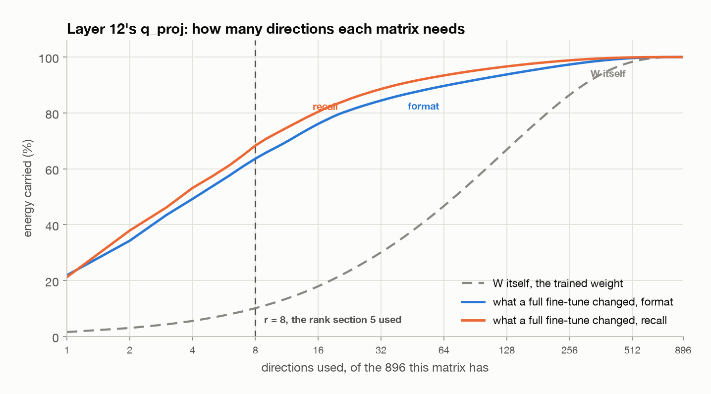
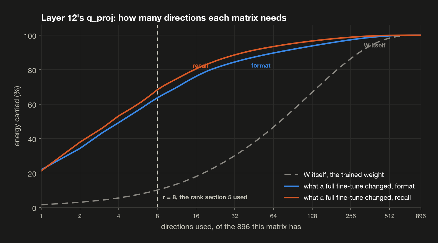
Take q_proj in layer 12, the matrix §2 walked through. It has 896 directions available to it.
The trained weight uses nearly all of them. It takes 299 directions to account for 90% of $W$, and its largest 8 hold just 10.1% of it. That’s what a dense, thoroughly trained matrix looks like, and it’s the reason you can’t simply compress $W$ itself to rank 8 and expect a working model.
The change a full fine-tune made to that same matrix is a different shape entirely. 90% of it fits in 68 directions for the format fine-tune and 38 for recall, four to eight times fewer than the weight it modifies. Its largest 8 directions hold 63.6% and 68.3% of it, against the weight’s 10.1%.
Layer 12 could be a lucky pick, so the demo measures every one of the 168 matrices the adapters sit beside, 24 layers of seven kinds (also why_the_update_is_low_rank):
1
2
3
4
5
6
7
8
9
10
11
12
13
14
15
16
17
18
19
20
  Every layer: directions for 90%, median over the 24 layers
  (smallest-largest):

  matrix          W itself  change, format  change, recall
  ----------------------------------------------------------
  q_proj      288 (55-331)     60 (29-120)      36 (18-51)
  k_proj        70 (21-81)      33 (17-44)      23 (10-29)
  v_proj      101 (71-109)      43 (26-54)      34 (22-43)
  o_proj     311 (186-389)     56 (14-116)      42 (25-57)
  gate_proj  640 (623-678)    204 (77-270)    122 (55-146)
  up_proj    666 (643-699)    187 (61-250)     93 (48-128)
  down_proj  632 (594-680)    198 (19-281)    106 (41-140)

  All 168 adapted matrices at once:

                  need > 8 for 90%   range  top-8 median
  --------------------------------------------------------
  W itself              168 of 168  21-699          7.8%
  change, format        168 of 168  14-281         62.7%
  change, recall        168 of 168  10-146         61.1%
Each cell is the median over the 24 layers, with the smallest and largest in brackets. Layer 12 is typical: its q_proj change needed 68 and 38 directions, and the medians across all 24 layers are 60 and 36. The bottom table is the one that settles it. Every one of the 168 changes, on both tasks, needs more than 8 directions to carry 90% of its energy. The lowest-rank change anywhere in the model still needs 10.
So the hypothesis is half right, and the half that’s wrong is the interesting half.
The change really is far more concentrated than the weight it modifies. Across all 168 matrices the largest 8 directions hold a median of 62.7% of the format change and 61.1% of the recall change, against 7.8% of the weight. That much is not subtle, and it’s the part of the low-rank story that holds up.
But it is not rank 8, and it isn’t close. If LoRA’s job were to reproduce what a full fine-tune does, rank 8 would capture around three fifths of it and miss the rest.
The resolution is that reproducing the full fine-tune was never the job. A full fine-tune finds one way to solve the task, out of many, and it has no reason to look for a tidy one: every direction is free to it, so it uses them. LoRA is asked a different question, whether there’s a rank-8 change that solves the task, and §5 answers it by finding one. “The update is low-rank” is the wrong claim. “A low-rank update suffices” is the right one, and only the second is what the measurements support.
That distinction stops being academic as soon as a task gets harder. Biderman et al. measured the same gap at real scale and found it matters: fine-tuning on programming and mathematics, “full finetuning learns perturbations with a rank that is 10-100X greater than typical LoRA configurations”, and in those settings LoRA “substantially underperforms full finetuning”. The compensation they report is on the other side of the ledger, and it follows from the same constraint: LoRA “better maintains the base model’s performance on tasks outside the target domain”, because a change restricted to a few directions is a change that disturbs less of what was already there. This post’s two tasks are both easy enough that the gap never bites. That is a fact about the tasks. The forgetting half can be measured here, and the end of this section does.
Two smaller results in those tables.
The MLP’s updates are markedly higher-rank than attention’s. Across all 24 layers of the format fine-tune, attention’s four kinds of matrix have medians of 33 to 60 directions for 90% of their change; the MLP’s three have 187 to 204. That isn’t just because k_proj and v_proj are narrow: q_proj and o_proj have the same 896 directions available as the MLP’s matrices, and their changes still need only 60 and 56. The recall fine-tune shows the same split at lower numbers. So “how low-rank is the update” isn’t one number for a model, it’s a number per kind of matrix, and the wide ones are the stubborn ones. That bears directly on where adapters should go, and §5 points the same way: adapters on the MLP alone did as well as adapters on all seven, while attention alone at rank 8 fell well short.
And depth changes the answer, for the weight as much as for the change. Here is q_proj at four depths, from the same why_the_update_is_low_rank:
1
2
3
4
5
6
  q_proj    W itself  change, format  change, recall
  ----------------------------------------------------
  layer 0         55              29              18
  layer 8        321              90              50
  layer 16       191              30              26
  layer 23       239              44              35
Layer 0’s weight needs only 55 directions for 90% of itself, against 321 at layer 8 and 239 at the last layer: the first layer’s weight is a simpler object than the ones above it. Its change is the lowest-rank of the four too, at 29 directions for format and 18 for recall. Nothing in that column suggests one rank is right for every layer, which is what per-layer rank allocation methods such as AdaLoRA exist to exploit.
A last note on what this measurement is not. Shuttleworth et al. run a spectral analysis that sounds similar and asks something different: they look at the singular vectors of the resulting weight matrix, not of the change, and find that LoRA introduces “new, high-ranking singular vectors, which we call intruder dimensions” that a full fine-tune doesn’t, then show by intervening on them that those dimensions cause forgetting. That’s a claim about how the two methods differ in where they leave the model, and this section’s measurement, which is about the shape of the change a full fine-tune makes, neither supports nor contradicts it. They’re worth reading together, and easy to conflate.
What the fine-tunes forgot
Biderman et al.’s title makes two claims, learns less and forgets less, and so far this section has only tested the first. The second can be measured with what §4 set up: score each fine-tune on post 4’s passage, which neither task resembles, and see how far it moved from the untrained model’s 20.87 (what_it_forgot):
1
2
3
4
5
6
7
8
9
10
11
12
  model                   exact match  passage  vs untrained
  ------------------------------------------------------------
  untrained                              20.87
  LoRA r=8, format           40 of 40    21.28         +1.9%
  full fine-tune, format     40 of 40    21.17         +1.4%
  LoRA r=8, recall           40 of 40    22.51         +7.9%
  full fine-tune, recall     40 of 40    22.08         +5.8%

  'passage' is perplexity on post 4's 550 tokens of prose, the same
  text and the same measure post 4 scored quantization with. Lower
  is better. LoRA ran at lr 0.0002 and the full fine-tunes at
  lr 1e-05, 200 steps each.
Every model in the table learned its task completely, 40 of 40, so a difference in the passage column isn’t a difference in how well the task was learned.
On these tasks, LoRA did not forget less. On format the two land a tenth of a point apart, 21.28 against 21.17. On recall the rank-8 adapter moved the passage more than the full fine-tune did, +7.9% against +5.8%. Each method ran at the learning rate it needs, and that condition matters. At LoRA’s rate, §4 showed the full fine-tune taking the passage to 2,291,268. At its own small learning rate, the full fine-tune disturbed the passage only a little.
Two things keep this from contradicting Biderman et al. Their fine-tunes ran on billions of tokens of programming and mathematics, far enough to move a model a long way; these ran 200 steps on toy tasks, where neither method moves it far. And §5’s passage column shows the variable their result turns on: forgetting climbs with rank, from 21.60 at rank 1 to 25.39 at rank 32 on recall. A lower-rank adapter forgets less than a higher-rank one, here as there. What a model this small, trained this briefly, can’t show is how rank 8 compares with a full fine-tune pushed hard enough for the difference to matter.
7. Merging, and the cost of not merging
An adapter’s update is the same shape as the matrix it modifies, which has a consequence: you can add it in and throw the adapter away.
\[W' = W + \frac{\alpha}{r}BA\]$W’$ is an ordinary 896 × 896 matrix. Nothing about it says it was ever adapted. Load a model whose weights are all $W’$ and it has no adapters, no extra matrices, and no extra multiplies, so it runs at exactly the speed the base model ran at. This is what Hu et al. mean in §4.1 when they say LoRA introduces no additional inference latency “by construction”, and it’s the property that distinguishes LoRA from the adapter methods that came before it, which inserted new layers that had to be run.
The demo merges all 168 adapters and checks that the model still computes the same thing (merging):
1
2
3
4
5
6
7
8
  check                                     result
  --------------------------------------------------
  adapters folded into their base weight       168
  largest logit difference                6.58e-05
  largest logit, for scale                 25.1507
  difference as a share of that            2.6e-06
  same next token                              yes
  weight change after merge then unmerge  0.00e+00
All 168 adapters fold in, and the model’s prediction survives it. The largest logit moves by a few parts in a million of its own size, and the token the model predicts doesn’t change.
That residue is floating-point noise, of exactly the kind post 3 measured when tiled attention agreed with the fused kernel to about 1.4e-6. It has the same cause, too: adding $BA$ into $W$ and then multiplying is the same arithmetic as multiplying separately and adding afterwards, but not in the same order, and floating-point addition doesn’t promise those agree to the last bit.
The reverse operation is how a serving system switches tasks: subtract the update and the base model is back. It isn’t exactly the inverse, though. Merging adds a number and unmerging subtracts the same number, and in floating point that round trip doesn’t always land on the bit you started from. The receipt’s last line measures how far off it lands, and on this run the answer is not at all: layer 12’s q_proj, the matrix it checks, came back to the bit. That’s luck of the particular numbers rather than a guarantee, since whether adding and then subtracting a value returns the original depends on how the two sizes round against each other. It’s why a system that swaps adapters thousands of times keeps a clean copy of $W$ rather than unmerging repeatedly.
Merging also changes the speed, and the timings below are from the same program, in two settings. Prefill is reading a prompt: 8 sequences of 256 tokens in one pass. Decode is generating: 8 sequences each adding one new token, which is what every step of a reply costs (forward_timings, printed by merging).
1
2
3
4
  forward pass, ms         merged  separate  separate / merged
  --------------------------------------------------------------
  prefill, 8 x 256 tokens   840.8    1014.8              1.21x
  decode, 8 x 1 token        34.8      40.5              1.16x
Keeping the adapters separate costs 1.21× a merged pass on prefill and 1.16× on decode. Those are wall clock, so the digits move between runs, but the direction won’t: an unmerged adapter does two extra matrix multiplies in each of 168 places, and a merged one does none. Each extra multiply is small, 8 numbers wide in the middle, but there are 336 of them, and on a model this small they are a real share of the work.
So merging is free at inference and costs a one-off pass over the weights. The only reason not to merge is that you have more than one adapter, which is §8.
8. Fifty fine-tunes of one base model
Here’s the situation LoRA is actually deployed for. You have one model and fifty customers, each wanting it adapted to their own data. A full fine-tune gives you fifty models. The memory arithmetic, from fifty_finetunes:
1
2
3
4
5
6
7
8
9
10
11
12
13
  step                                    result
  -------------------------------------------------------------
  one full copy of the model       1,976,131,072        bytes
  x 50 fine-tunes, kept whole     98,806,553,600        bytes
  / 1,073,741,824 bytes in a GiB            92.0          GiB

  one adapter, r=8                    17,596,416        bytes
  / 1,048,576 bytes in a MiB                16.8          MiB
  x 50 adapters                      879,820,800        bytes
  + one shared base model, total   2,855,951,872        bytes
  / 1,073,741,824 bytes in a GiB            2.66          GiB

  whole copies / shared base               34.6x  more memory
92.0 GiB against 2.66 GiB, a factor of 34.6. Fifty whole models need more memory than an 80 GB GPU has; one model and fifty 16.8 MiB adapters barely notice each other. That ratio is the main serving argument for LoRA, and it gets better with the number of adapters, since each new customer costs 16.8 MiB instead of 1.84 GiB.
The catch is the one §7 set up. You can only merge one adapter at a time. Merging customer A’s update into $W$ produces a model that is customer A’s, and a request from customer B now has to unmerge it and merge a different one, which is a pass over 358 million parameters between requests. That’s fine if requests arrive in long runs per customer, and useless if they interleave.
So a real multi-tenant server keeps every adapter unmerged and pays the extra multiplies on every forward pass, which is the cost §7 measured. It also means the batch can no longer be one matrix multiply: tokens belonging to different customers need different $A$ and $B$, so the adapted part of the layer becomes a grouped multiply, one group per adapter in the batch. S-LoRA is built around exactly this, keeping adapters in host memory, fetching the ones a batch needs, and using custom kernels to batch the heterogeneous part.
Here’s what that looks like at one matrix, for the batch the demo runs below:
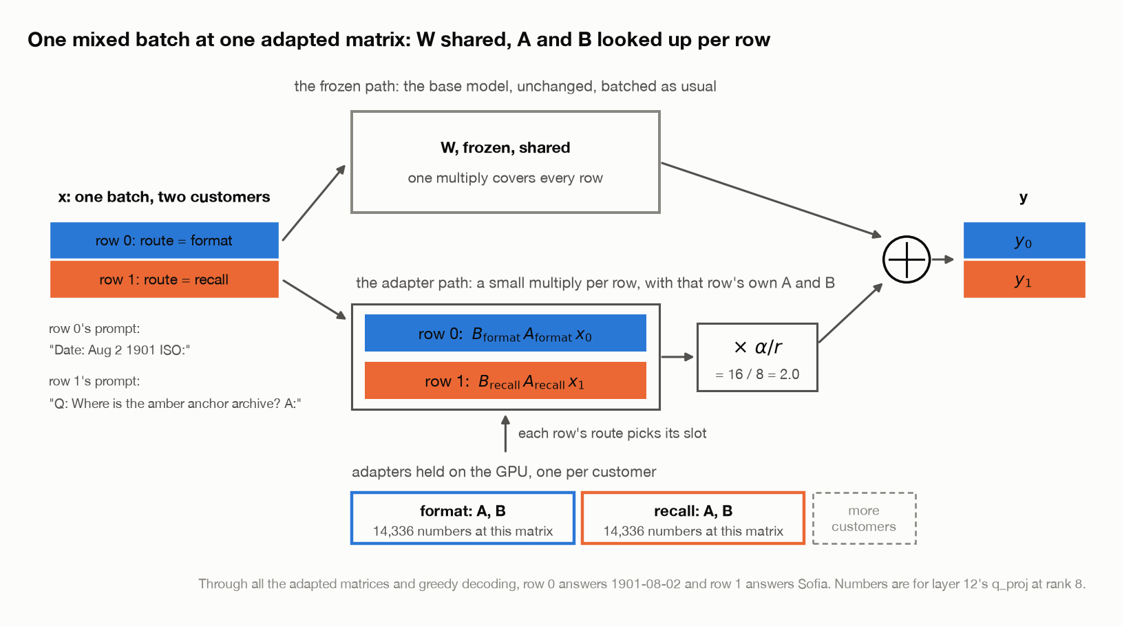
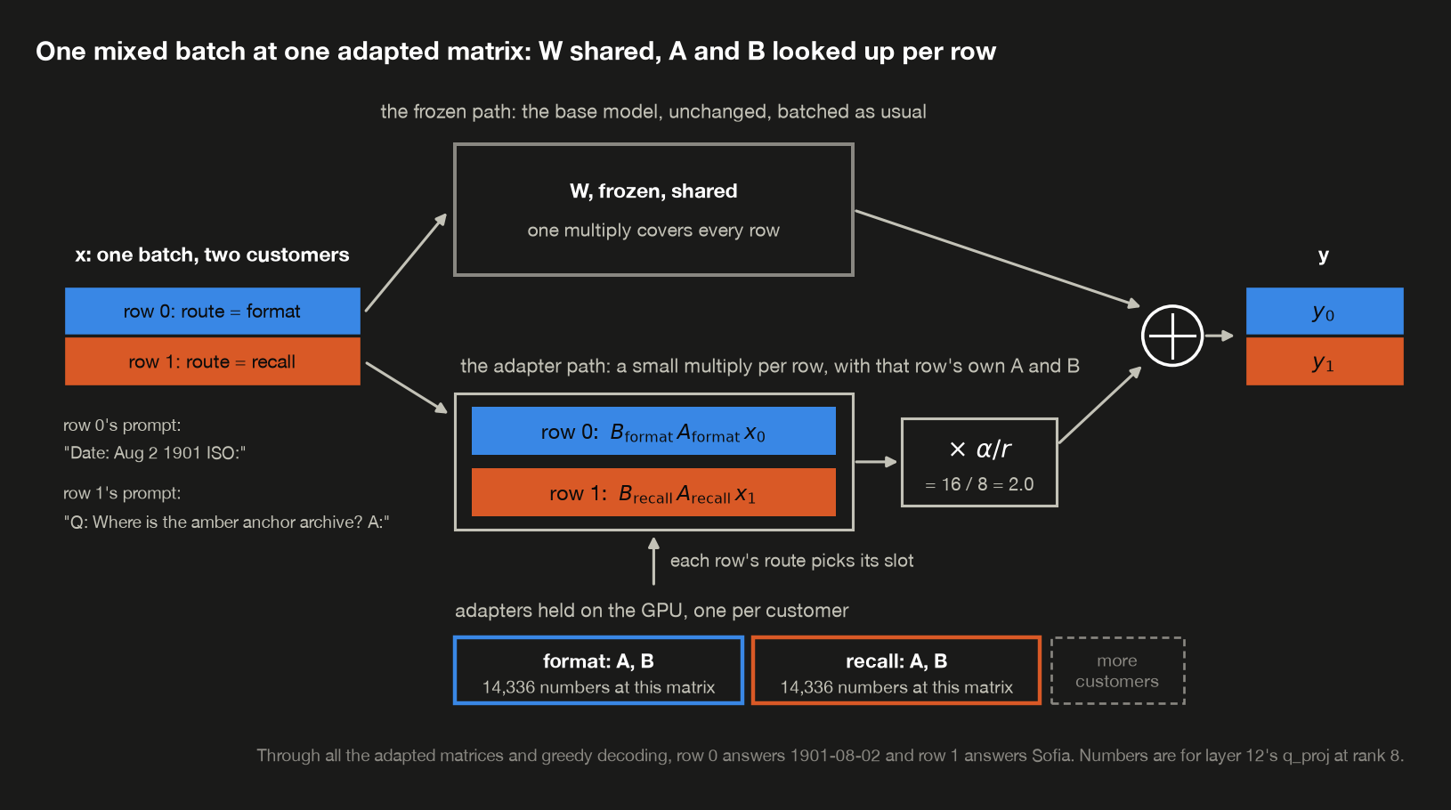
Both rows go through $W$ together, so the expensive multiply is still one multiply, however many customers share the batch. Only the thin path is split up. Each row carries a route naming its adapter, and at every adapted matrix the route picks that adapter’s $A$ and $B$ out of the ones held on the GPU. The two results are scaled by $\alpha/r$ and added back row by row, exactly as in §2.
The demo does it the simplest correct way. It loads the rank-8 adapters §5 trained for both tasks beside one copy of the base model, and puts a format prompt and a recall prompt in the same batch, each row routed to its own adapter. At every adapted matrix it gathers each row’s $A$ and $B$ and multiplies them batch by batch (MultiLoRALinear, one_batch_two_customers):
1
2
3
4
5
6
7
8
9
10
11
12
13
  row's adapter    expected       alone  mixed batch       swapped
  ------------------------------------------------------------------
  format         1901-08-02  1901-08-02   1901-08-02  10000-1 A. 1
  recall              Sofia       Sofia        Sofia    2019-09-01

  'alone' is that adapter served by itself; 'mixed batch' is both
  rows in one forward pass, each routed to its own adapter;
  'swapped' is the same batch with the two routes exchanged.

  forward pass, ms         merged  separate   mixed  mixed / merged
  -------------------------------------------------------------------
  prefill, 8 x 256 tokens   840.8    1014.8  1037.7           1.23x
  decode, 8 x 1 token        34.8      40.5    42.3           1.22x
Both rows give the answer their own adapter gives when served alone, and both are right. The swapped column is the control: the same batch with the two routes exchanged hands the date to the facts adapter and the question to the dates adapter, and both answers turn to nonsense. The answers come from the routing, not from the prompts.
The bottom table is the price. A mixed batch costs 1.23× a merged forward pass on prefill and 1.22× on decode, slightly more than one unmerged adapter, the difference being the gather. That’s the running cost behind the 34.6×: fifty customers fit in 2.66 GiB, and every forward pass they share takes about a fifth longer than one merged model’s would. S-LoRA’s custom kernels exist to shrink that fifth.
Post 5 ended on a version of this same shape, so put the two side by side. There, per-token sparsity was real and batch sparsity wasn’t, because a batch needs the union of what its tokens want. Here, the single-adapter saving is real and the multi-adapter saving is smaller than it looks, because a batch needs the union of what its requests want. Batching is where clean per-item stories go to be complicated.
Serving at scale
The demo routes two rows by hand, on one machine. A real server has three more questions to answer: who decides which adapter a request gets, what happens when that adapter isn’t on the GPU, and what changes when one GPU isn’t enough. The demo doesn’t measure any of this. What follows is how the serving systems describe themselves, in their documentation and papers.
The request names its adapter. vLLM doesn’t look at a prompt to work out which fine-tune it needs. Adapters are registered under names, and a request picks one in its model field, the same field that would otherwise name a model. If you want the choice made for the user, say by what kind of question it is, that’s a router you write and put in front: a rule or a small classifier that reads the request and fills in the name, and whatever time it takes is added to every request.
An adapter has to be on the GPU before a batch can use it. vLLM keeps adapters in two tiers. --max-loras sets how many different adapters one batch can use, and --max-cpu-loras how many it keeps cached in ordinary memory, ready to copy over. An adapter in neither has to be loaded from disk first, and the request for it waits. S-LoRA is built the same way: every adapter lives in host memory, the ones the current batch needs are copied to the GPU, and while one batch runs it reads the waiting queue to predict the next batch’s adapters and copies them early, so the copying overlaps the computation.
The cap on adapters per batch is where requests wait. --max-loras defaults to 1, so out of the box each batch serves one adapter, and a request for a different one waits for a later step. Raising it lets one batch mix more customers, which is what the demo above does with two. A higher --max-lora-rank, the largest rank the server will accept, costs more memory, so it’s set to the largest rank you actually serve.
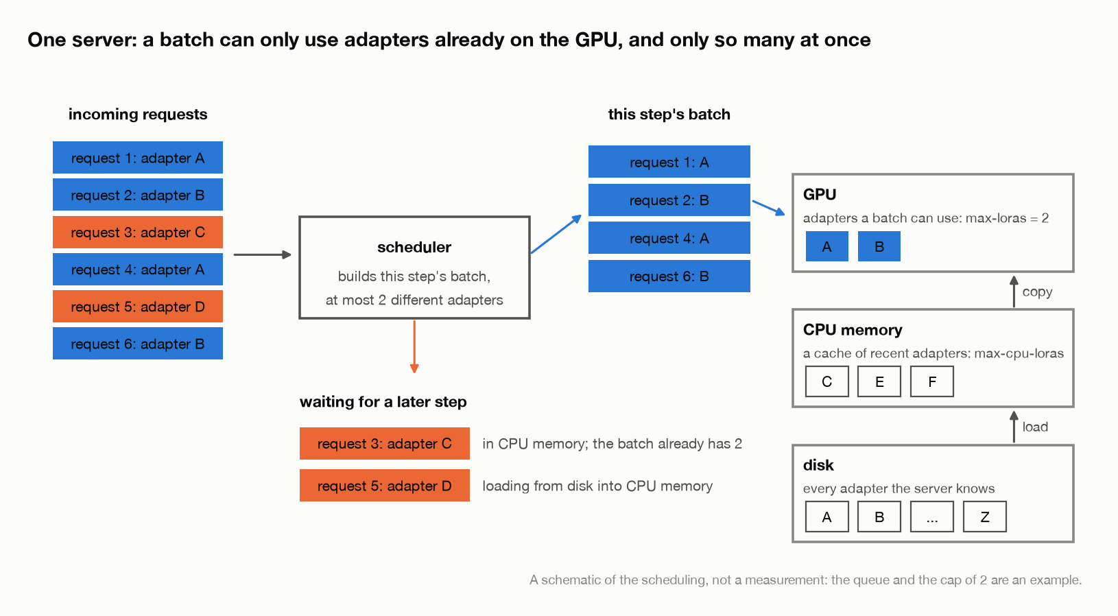
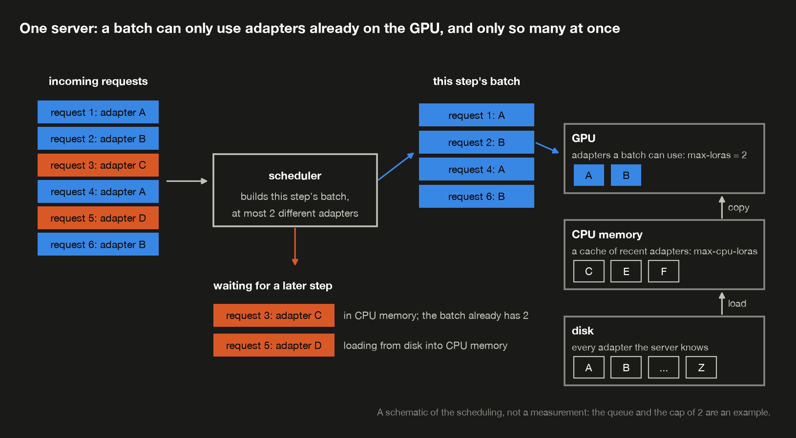
The figure follows six requests through one step, with the cap set to 2. Requests 1, 2, 4 and 6 name adapters A and B, which are already on the GPU, so they run together in one batch. Request 3 names C, which is sitting in CPU memory and could be copied over, but the batch already uses its two adapters, so it waits a step. Request 5 names D, which is only on disk, so it waits for the load. Neither wait has anything to do with how fast the forward pass is.
Faster kernels shrink the per-pass cost. The 1.23× and 1.22× above come from the demo’s plain gather. Punica wrote a GPU kernel that batches different adapters’ multiplies together, and reports 12× the throughput of the serving systems it compared against while adding about 2 ms of latency per token. Those are their numbers on their hardware, not this post’s.
More than one GPU. Two kinds of scaling combine, and adapters fit into both.
The first splits one copy of the model across GPUs. When the base model is too big for one GPU, each weight matrix is cut into pieces and each GPU multiplies by its own piece, which is called tensor parallelism. S-LoRA cuts each adapter’s $A$ and $B$ to line up with how the base matrix is cut, so each GPU applies its share of the adapter to its share of the work. The extra communication is a few exchanges per layer, which its authors call negligible next to the base model’s, because $r$ is far smaller than the model’s width. vLLM by default splits only half of the adapter computation this way, and --fully-sharded-loras splits all of it.
The second runs many copies of the server. To serve 1,000 requests at once you run several copies, each on its own GPU or group of GPUs, and a router spreads the requests across them. With adapters, the router should send a request to a copy that already holds the adapter it names, so that copy doesn’t load it again and its batches mix fewer adapters, while still steering around a copy that’s overloaded. Ray Serve’s model multiplexing works this way: the request names its model in a header, it goes to a copy that has that model loaded, or to another copy that loads it if those are overloaded, and each copy drops its least recently used model when it’s full. So popular adapters end up loaded on every copy, and rarely used ones get loaded wherever they’re asked for.
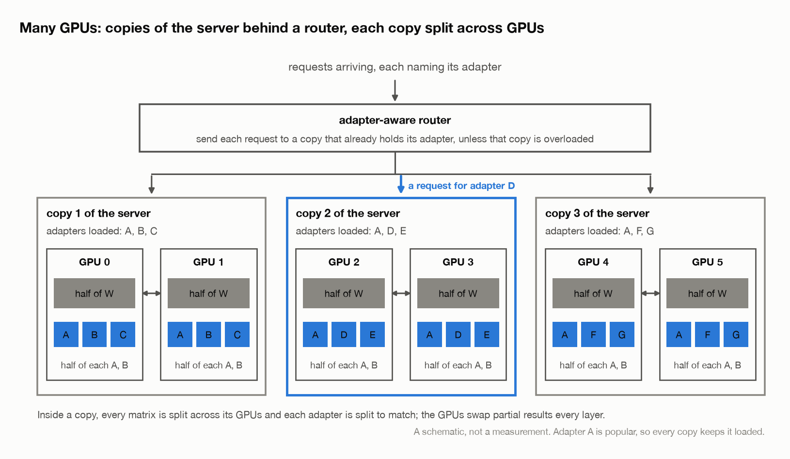
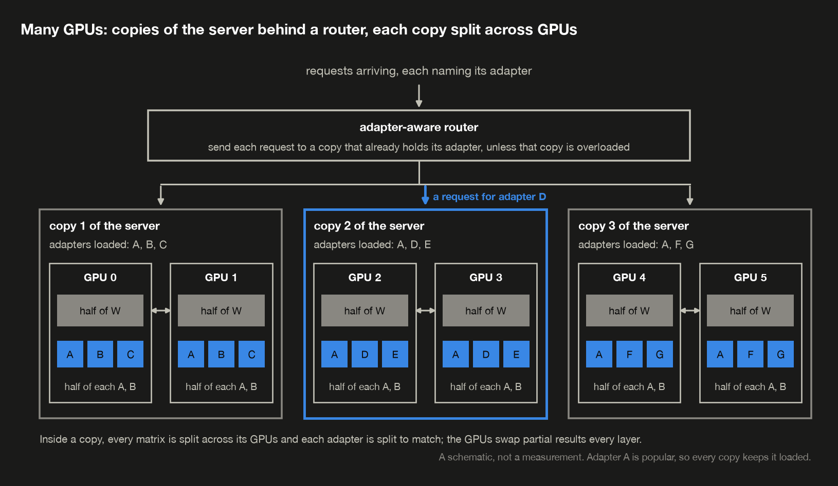
Read the figure from the top. A request for adapter D arrives, and the router sends it to copy 2, the one copy that has D loaded. Inside copy 2 the work is split across two GPUs, each holding half of every weight matrix and the matching half of every adapter it has loaded, and the two swap partial results at every layer. Adapter A is loaded on every copy because it’s popular; D, E, F and G each live on one. To handle more traffic you add copies, and the router’s job is to keep each copy’s batches to the adapters it already holds.
None of this changes the arithmetic at the start of this section. Each copy of the server still stores the base model once, each adapter still costs 16.8 MiB, and every forward pass that mixes adapters still pays for the extra multiplies.
9. What follows from all this
LoRA does not make the model cheaper to hold; it makes the update cheap. The frozen weights are still resident during training, so model-state memory (weights, gradients and optimizer moments) falls by 3.9× while the trainable parameter count falls by 112×. Post 5’s lesson in a new place: the number in the headline and the number on the invoice measure different resources.
What rank you need is a property of the task, not of the method. A rule that applies to every example was learned perfectly at rank 1. Sixty-four arbitrary facts kept getting firmer up to rank 16. Neither number transfers to your problem, and the useful move is to sweep, which is affordable: each run in §5 took about a third of a full fine-tune’s time per step and a quarter of its model-state memory. Run each rank more than once, too, because at this scale the seed moved exact match as much as rank did.
“The update is low-rank” is not what the measurement says. What a full fine-tune actually does to a matrix is high-rank. What §5 shows is that a low-rank update can reach the same behavior, which is a claim about the existence of a good solution, not about the shape of the one gradient descent finds unaided. Biderman et al. found the gap matters on programming and mathematics, tasks that ask far more of a model than these two toy ones.
And the serving story is the reason LoRA won. One base model plus a directory of 16.8 MiB adapters is a different operational shape from fifty copies of a model, and it’s why serving systems such as vLLM can run many adapters over one base model, across as many GPUs as the traffic needs (§8). The cost is that an adapter kept unmerged runs extra multiplies on every forward pass, and a batch that mixes adapters forces exactly that: LoRA’s “no additional inference latency” holds only once an adapter is merged.
10. Sidebar: the probe
One question to close on, the kind this material gets asked, and what separates an answer that sounds right from one that is.
“We need a fine-tune per customer, fifty of them. LoRA trains under 1% of the parameters, so training is about a hundred times cheaper and we can serve all fifty on one GPU. Right?”
The tempting answer: “Yes. 0.9% trainable is ~100× less memory, and the adapters are megabytes, so fifty of them is nothing.”
Both halves are half right, and they fail in different directions.
1. Separate trainable parameters from memory. The parameter count falls 112×; model-state memory falls 3.9×, from 7,538.3 MiB to 1,951.7 MiB, before activations, which neither number counts. What disappeared is the gradient and AdamW’s two moments, 12 bytes per trainable parameter in fp32. What did not is the weights, because a frozen parameter still has to be there for the forward pass. If the model didn’t fit before, LoRA may not be the thing that makes it fit.
2. And separate memory from time. A step got about three times faster here, not a hundred. The forward pass costs the same. The backward pass still has to carry the gradient through every frozen weight to reach the adapters, and got only 1.6× cheaper. Most of the saving is the optimizer update that no longer touches 494 million parameters.
3. Refuse “rank 8” as a default. This post’s two tasks disagree completely about what rank buys. A systematic rule was learned perfectly at rank 1. Sixty-four arbitrary facts kept improving up to rank 16, where rank behaved like room to store them. Each sweep run costs about a third of a full fine-tune’s step time and a quarter of its model-state memory, so measure rank rather than inherit it.
4. Then say what serving fifty actually costs. Fifty whole fine-tunes are 92.0 GiB of weights; fifty adapters over one shared base are 2.66 GiB, 34.6× less. That is real, and it’s the reason multi-adapter serving exists. The asterisk is that this only holds while the adapters stay unmerged, and an unmerged adapter costs extra work on every forward pass. A batch that mixes customers can’t merge any of them, which is the case production systems are built around (S-LoRA keeps adapters in host memory and batches them with custom kernels). And the request has to name its adapter, the server can only mix so many adapters per batch, and at scale a router has to send each request to a GPU that already holds its adapter (§8).
What the question is really testing is whether “1% of the parameters” is being read as one number that describes training cost, memory, latency and serving all at once, or as what it is: a statement about how many numbers receive a gradient.
What’s next
Post 7 is QLoRA, which is this post and post 4 at the same time: quantize the frozen base model to 4-bit, then train a LoRA adapter on top of it. Post 4 already derived the format it uses, NF4, to within 6e-08 of the shipped table, so the piece that’s new is the interaction. The questions there are what happens to gradients that have to flow back through quantized weights, why the adapter stays in higher precision when the thing it’s adapting doesn’t, and whether the two approximations compound or stay out of each other’s way. §1’s four copies is the number to keep in mind: QLoRA attacks the one this post left alone.
Appendix: counting the adapter parameters
This appendix derives §3’s census matrix by matrix, so every number in it can be checked by hand. One rule does all the work: an adapter on a matrix with $d_{in}$ inputs and $d_{out}$ outputs holds
\[r \times d_{in} \;+\; d_{out} \times r \;=\; r\,(d_{in} + d_{out})\]parameters, because $A$ has $r$ rows of $d_{in}$ numbers and $B$ has $d_{out}$ rows of $r$ numbers.
Qwen2.5-0.5B has 24 identical layers, each holding seven adapted matrices. Their shapes come from the model’s configuration: a width of 896, an MLP inner width of 4,864, and 14 query heads against 2 key/value heads of 64 numbers each, so the key and value projections produce $2 \times 64 = 128$ numbers rather than $14 \times 64 = 896$.
| matrix | $d_{in}$ | $d_{out}$ | $d_{in} + d_{out}$ | at $r = 8$ |
|---|---|---|---|---|
q_proj | 896 | 896 | 1,792 | 14,336 |
k_proj | 896 | 128 | 1,024 | 8,192 |
v_proj | 896 | 128 | 1,024 | 8,192 |
o_proj | 896 | 896 | 1,792 | 14,336 |
gate_proj | 896 | 4,864 | 5,760 | 46,080 |
up_proj | 896 | 4,864 | 5,760 | 46,080 |
down_proj | 4,864 | 896 | 5,760 | 46,080 |
| one layer | 22,912 | 183,296 |
One layer’s seven matrices sum to $22{,}912$ in the $d_{in} + d_{out}$ column, and 24 layers make $24 \times 22{,}912 = 549{,}888$. That number is the adapter’s size per unit of rank, which is why every row of §5’s sweep is a multiple of it: rank 1 is 549,888 parameters, rank 8 is $8 \times 549{,}888 = 4{,}399{,}104$, and rank 32 is $32 \times 549{,}888 = 17{,}596{,}416$. An adapter’s size is exactly linear in its rank.
In bytes, at 4 bytes per fp32 number:
\[4{,}399{,}104 \times 4 = 17{,}596{,}416 \text{ bytes} = 16.78 \text{ MiB}\]And what the adapters leave alone, which is the model’s 494,032,768 parameters minus the 357,826,560 they sit beside:
| not adapted | parameters |
|---|---|
| embedding table, tied to the output head | 136,134,656 |
| norm weights, 2 norms per layer plus the final one, 896 each | 43,904 |
bias vectors on q_proj, k_proj, v_proj | 27,648 |
| total | 136,206,208 |
$357{,}826{,}560 + 136{,}206{,}208 = 494{,}032{,}768$, which is the model, so nothing is unaccounted for.
Appendix: all notation
The terms and symbols this post leans on; anything not listed is defined where it first appears. Post 1’s appendix covers attention’s notation, post 2’s the memory and serving terms, post 4’s the quantization formats, and post 5’s the mixture-of-experts terms.
| Symbol | Means | In this post’s runs |
|---|---|---|
| $W$ | a weight matrix the model shipped with, frozen during LoRA training | e.g. $(896, 896)$ |
| $A$, $B$ | the adapter’s two trainable matrices, $A$ narrowing and $B$ widening | $(8, 896)$ and $(896, 8)$ |
| $r$ | the rank: the width of the bottleneck between $A$ and $B$ | 1 to 32 in §5, 8 elsewhere |
| $\alpha$ | the constant scaling the update, always $2r$ here so $\alpha/r$ is fixed | 16 at $r = 8$ |
| $\Delta W$ | the change to a weight matrix: $(\alpha/r)BA$ for LoRA, $W_{after} - W_{before}$ for a full fine-tune | $(896, 896)$ |
| rank | how many independent directions a matrix holds, at most its smaller side | 8 for an adapter, up to 896 for $W$ |
| singular value | how far a matrix stretches along one of its independent directions | 8 non-zero for a rank-8 update |
| energy | the sum of the squares of a matrix’s entries; it equals the sum of its singular values squared, so each direction carries a share of it | §6’s measure |
| directions for 90% | the fewest directions whose squared singular values reach 90% of the energy | §6’s first table |
| full fine-tune | training every parameter, the thing LoRA is an alternative to | 494,032,768 trainable |
| adapter | the trained $A$ and $B$ for every adapted matrix, saved as one file | 4,399,104 parameters, 16.8 MiB |
| merging | folding $(\alpha/r)BA$ into $W$, after which no adapter is left to run | §7 |
| loss | $-\log p$ for the probability $p$ given the correct next token, averaged over the graded positions; lower is better | 6.93 at the start of §4’s runs |
| gradient | one number per trainable parameter, saying how to change it | same size as the trainable set |
| AdamW moments, optimizer state | the optimizer’s two running averages, one number each per trainable parameter | 2 more copies |
| training state | gradient plus both moments: 12 bytes per trainable parameter in fp32 | 5,653.8 MiB full, 50.3 MiB LoRA |
| model state | weights plus training state; what §4’s memory table counts, leaving out activations and other runtime memory | 7,538.3 MiB full, 1,951.7 MiB LoRA |
| GQA | grouped-query attention: fewer key/value heads than query heads | 14 query, 2 key/value |
| exact match | how many of the 40 test prompts get exactly the right answer under greedy decoding, after trimming spaces at the ends; unseen dates for format, trained facts for recall | §4 and §5’s score |
| seed | the fixed starting point of a random-number generator; here, what $A$’s random start is drawn from | 0, 1 and 2 in §5 |
| perplexity | how many tokens a model is, on average, torn between when predicting a passage; lower is better | 20.87 untrained, on post 4’s passage |
| prefill, decode | reading a whole prompt in one pass, against generating one new token per sequence | §7 and §8’s two timings |
| mixed batch | one batch whose rows belong to different adapters, so none of them can be merged | §8 |
References
- Hu et al., LoRA: Low-Rank Adaptation of Large Language Models (2021) — the method this post implements. §4.1 is the source of the $\alpha/r$ scaling and of the merging argument (“this guarantees that we do not introduce any additional latency during inference compared to a fine-tuned model by construction”), which §7 measures. Their main GPT-3 experiments adapt only $W_q$ and $W_v$; §7.1 reports that adapting both beats adapting either alone. §7.2 is the finding §5 revisits: “a rank as small as one suffices for adapting both $W_q$ and $W_v$ on these datasets”, on GPT-3 with WikiSQL and MultiNLI.
- Aghajanyan, Zettlemoyer and Gupta, Intrinsic Dimensionality Explains the Effectiveness of Language Model Fine-Tuning (2020) — the prior result LoRA’s low-rank hypothesis is built on, cited in its §1.
- Biderman et al., LoRA Learns Less and Forgets Less (2024) — the counterweight to §5’s easy case, and the direct corroboration of §6. On programming and mathematics, in both instruction tuning and continued pre-training on 20B tokens, LoRA “substantially underperforms full finetuning” while better preserving performance outside the target domain. Their measurement of the update is the one §6 reproduces at laptop scale: “full finetuning learns perturbations with a rank that is 10-100X greater than typical LoRA configurations.” §6’s last subsection measures the forgetting half on this post’s tasks, where it does not reproduce.
- Shuttleworth et al., LoRA vs Full Fine-tuning: An Illusion of Equivalence (2024) — a different spectral measurement from §6’s, and worth not conflating with it. They analyze the singular vectors of the resulting weight matrix rather than of the change, and find LoRA introduces “new, high-ranking singular vectors, which we call intruder dimensions” that full fine-tuning does not, then show by intervening on them that they cause forgetting.
- Dettmers et al., QLoRA: Efficient Finetuning of Quantized LLMs (2023) — post 7’s subject, and the source of §3’s target list: they report that “LoRA on all linear transformer block layers are required to match full finetuning performance”, having found query and value alone insufficient on LLaMA 7B with Alpaca. §5 tests the choice on this post’s model.
- Sheng et al., S-LoRA: Serving Thousands of Concurrent LoRA Adapters (2023) — §8’s problem solved at production scale. Adapters are kept unmerged and stored in host memory, fetched per query, with custom kernels for batching heterogeneous adapters; they report up to 4× the throughput of the baselines and “several orders of magnitude” more served adapters. §8’s serving subsection also draws on its §5, which prefetches the next batch’s adapters from the waiting queue, and its §6, which splits each adapter to match a tensor-parallel base model and calls the added communication negligible.
- Chen et al., Punica: Multi-Tenant LoRA Serving (2023) — a GPU kernel that batches many adapters’ multiplies over one copy of the base model; the abstract reports 12× higher throughput than the serving systems it compares against, “only adding 2ms latency per token”.
- vLLM, LoRA Adapters and engine arguments (documentation) — a request names its adapter in the
modelfield;--max-lorasis the “max number of LoRAs in a single batch”, default 1;--max-cpu-lorasthe number kept in CPU memory;--fully-sharded-lorasshards the whole adapter computation under tensor parallelism, where the default shards half. - Ray, Model Multiplexing (Ray Serve documentation) — routing by a model ID in the request header to replicas that already have that model loaded, with least-recently-used eviction per replica.
- Kalajdzievski, A Rank Stabilization Scaling Factor for LoRA (2023) — argues the $\alpha/r$ scaling this post uses under-scales high ranks, and proposes $\alpha/\sqrt{r}$ instead. Relevant to §5’s rank-32 row, which needed three times the steps to catch up.
- Hugging Face, GPU memory usage (Transformers documentation) — backs §4’s caveat that the memory table counts model state only. It breaks training memory into weights, optimizer states, gradients, forward activations, temporary tensors and other overhead, and gives mixed precision as 6 bytes of weights, 8 of Adam moments and 4 of fp32 gradient per parameter, one of the setups §4 notes would change its arithmetic.
- Qwen Team, Qwen2.5 Technical Report (2024) — the model fine-tuned throughout, the same checkpoint post 4 quantized.