LLM Architecture Refresh [8]: Learning from Rewards
What happens when we train a language model using rewards instead of correct answers? In this post, I implement Group Relative Policy Optimization (GRPO) from scratch using Qwen2.5-0.5B-Instruct and LoRA. The model generates multiple solutions to multiplication problems, receives rewards from a programmatic verifier, and learns by comparing its attempts. I train it from three random seeds, and three more times with each group's rewards shuffled, to separate what the reward taught from what the training loop does on its own, and look at how RLHF runs the same loop with a learned judge in place of a program.
My highlights: key concept insight takeaway pitfall open question try this. The notes beside them are my own asides; on a phone, tap note to read one.
The first post without an answer key
For the first seven posts in this series, whenever I trained a model, I showed it what the right answer looked like. This time, I want to try something different: tell the model only whether its answer is correct, and let it figure out how to improve.
Most of those posts didn’t train anything. Posts 1 to 5 were about running a model and what that costs: a transformer block taken apart, keys and values cached, attention computed in tiles, weights stored in fewer bits, and a model that runs only some of its parameters for each token. Post 6 and post 7 did train something, a small adapter beside a frozen model and a small connector that joins a frozen image encoder to a frozen language model, and both trained it the same way. Every example came with a target: a fact for post 6, and for post 7 a caption like a red square or the answer three to “How many shapes are there?”. The loss measured how far the model’s next token was from it. That’s supervised learning: learning from target outputs someone wrote down.
For a lot of tasks, though, it’s easier to check an answer than to write down the one right way to reach it. A program can tell whether a product came out right, whether code passes its tests, or whether a meeting ended up on the calendar, without anyone demonstrating the steps. Reinforcement learning (RL) learns from that kind of check. The model acts, gets a score for the outcome, and training pushes it toward whatever scored well, with no target to copy.
This post builds one version of that loop by hand, on a laptop, with a task small enough to watch: two-digit multiplication. The model writes several answers to each question, a program scores each one 1 if it’s right and 0 if it isn’t, and the model is pushed toward the answers that beat its other tries. I also train it three times, each from a different random seed (the number that sets a run’s starting adapter weights and the answers it samples), and three more times with each question’s rewards shuffled among its answers, because seeing accuracy go up isn’t enough. I want to know whether the model is actually learning from the reward.
That leaves two questions. Can a score of 1 or 0, with no answer to copy, make a small model better at problems it never trained on? And if it can, how do we tell what the score actually taught?
The short version
Can a small language model learn from a right-or-wrong score, without ever being shown the right answer?
I took Qwen2.5-0.5B-Instruct, a small chat model, and asked it to multiply two-digit numbers. Out of the box, before any training here (the untrained model from now on), it gets 37.5% of 200 test problems right (§2). Then I trained it with GRPO (Group Relative Policy Optimization), the method DeepSeek used for its math and reasoning models, with the sampling, the scoring and the update written out by hand rather than imported from an RL library. For each question the model writes eight answers, a program gives each a 1 if it’s the right integer and a 0 otherwise, and each answer is compared with its own group’s average: the ones above it are made more likely, the ones below less (§4, §5). Only a LoRA adapter trains, a small set of weights beside the frozen ones, as in post 6.
After 60 training steps, three runs with different random seeds reached 50.5%, 59.0% and 57.0% accuracy on the same 200 unseen problems, up from the untrained model’s 37.5%.
But how much of that improvement came from learning which answers were correct, rather than simply changing the model through training?
To test this, I ran a control experiment. Everything stayed the same, except I shuffled the rewards among the eight answers in each group. The model still received positive and negative feedback, but that feedback no longer said which answers were right.
The controls improved too, reaching 47.0%, 42.0% and 42.0%. That’s a gain of 4.5 to 9.5 points. Training on shuffled rewards still changes the model.
What matters is the difference: real-reward training gained 13.0 to 21.5 points, and even its weakest run outperformed the strongest shuffled-reward control. This is evidence that the model learned from the relationship between its answers and their rewards, not merely from undergoing additional training. The controls also remind us that an improvement in test accuracy, by itself, doesn’t establish what the model learned (§6, §7).
The same runs also showed where learning from a group’s scores runs thin:
- The model has to find a right answer first. Training can only push toward a right answer if one of the eight tries found it. Before training, the model often got a problem right on some try even when its single best guess was wrong, and those problems are where training has something to work with. An update changes weights that every problem shares, though, so it can also reach problems where no try was right, and the test problems it never trains on (§2, §7).
- Most groups teach nothing. Each answer is pushed by how far its score sits from its group’s average. When all eight answers are right, or all are wrong, every score equals the average, so no answer gets any push. Before training, that was true of most groups (§4).
- The training reward was a poor guide. In one run (seed 0), the average reward during training hardly moved after the first ten steps, while the model’s accuracy on the test problems went up clearly (§6).
- The seeds landed far apart. The three runs differ only in their seed, and one gained a good deal less than the other two. With three runs, all I can report is the range they cover, which isn’t a precise size for the effect. They show that training on the real reward helped, and helped more than the shuffled-reward control, but not by exactly how much (§6).
- What improved was mostly the arithmetic. Most of the problems seed 0 newly got right had been answered with a wrong number before; only a few had been something other than a plain number. Most were also problems the untrained model had already got right on at least one of its eight tries. So training mostly taught the model to give, as its first answer, a product it could already sometimes write. That doesn’t show it learned a general way to multiply (§7).
RLHF, reinforcement learning from human feedback, puts a model trained on people’s preferences where this post’s program is. It’s a bigger recipe than this loop, with fine-tuning and a learned reward model before the RL step, and the best-known version trains with PPO (Proximal Policy Optimization), an older method that uses a second network where GRPO uses groups. DeepSeek-R1’s authors explain why they’d rather trust a program wherever one can check the answer (§8).
None of this makes a good calculator, and it isn’t meant to. Multiplication is here because the reward is unambiguous and cheap, so every number below can be checked.
Setup
Everything below is measured, and you can re-run all of it:
1
2
3
git clone https://github.com/bearbearyu1223/llm-architectures-refresher
cd llm-architectures-refresher
uv sync && uv run demo08
The code is in demos/d08_rewards.py. There’s no RL library in it: the sampling, the reward, the group comparison and the loss are all written out, and the loss itself is one function, grpo_objective. The adapters are post 6’s lora.py. Every number this post quotes is printed by that program (§2’s table of how a sampling setting changes the model’s probabilities by uv run demo08 --temperature, §5’s table of the penalty for drifting from the starting model by uv run demo08 --kl-table, §8’s reward-model example by uv run demo08 --reward-model), and each block of its output, which I call a receipt, names the function that printed it.
The demo trains six times, and on my Mac the whole run took about an hour by the clock. That’s a rough figure rather than a receipt, since the program prints its timings only to its progress output, not to the captured receipts. uv run demo08 --quick runs every section at toy size, to check that it works before committing the time.
The model. Qwen2.5-0.5B-Instruct is the instruction-tuned version of the Qwen2.5-0.5B that posts 4, 6 and 7 used (the report). Instruction-tuned means it was trained further, after pretraining, to answer questions in a chat format, which is what this task needs: a base model asked “What is 23 × 47?” is as likely to continue the text as to answer it. It’s small enough to train on a laptop in fp32, four bytes per number as in posts 6 and 7, and the frozen reference copy that training needs costs no extra memory (§5 explains both).
The task. Each question is “What is a × b? Answer with just the number.”, with a and b between 10 and 99. The 256 training problems and 200 test problems don’t overlap: if 23 × 47 is in training, neither 23 × 47 nor 47 × 23 is in the test set. The demo’s opening lines, from main:
1
2
3
4
5
6
  model                              Qwen/Qwen2.5-0.5B-Instruct
  precision                          float32
  task                               a x b, a and b in 10..99
  reward                             1 if the answer is the right integer
  format-valid                       a lone integer: 1081, 1,081 or 1081.
  train / test problems              256 / 200, disjoint
The reward is the score an answer gets: 1 if the answer is the right integer, 0 for anything else. Format-valid means the answer is a lone integer, so the program can read a number out of it at all. 1081, 1,081 and 1081. are format-valid; = 1081 and 23 x 47 = 1081 aren’t, so they score 0 even when the number in them is right. That’s a deliberate choice, and §7 shows what it did.
Seeds. Each training run starts from a fixed seed, the number that sets its random starting adapter weights and the answers it happens to sample, so rerunning the demo on the same machine prints the same results. A different machine can sum floating-point numbers in a different order, and sampling turns tiny differences into different answers, so expect different scores there. That’s why §6 trains with three seeds and reports all three.
Table of Contents
The short version above has the findings without the derivations.
- What next-token training measures
- A task with a checkable answer
- From rewards to a gradient
- Groups instead of a value model
- One update by hand
- Training it
- What it actually learned
- Where RLHF fits
Then what’s next and all notation at the end.
1. What next-token training measures
Before training on a score, I want to be exact about what training on an answer does. Supervised learning and RL both work by changing the probabilities a model gives the tokens of an answer. They differ in where that answer comes from, and in what decides whether it should become more likely or less likely.
A language model doesn’t produce an answer in one go. It produces one token at a time, and at each step it gives every token in its vocabulary a probability of coming next. A token’s log-probability (log-prob) is the natural logarithm of the probability the model gave that token, given everything before it. Probabilities are between 0 and 1, so log-probs are 0 or negative: a log-prob of 0 means the model was certain, and the more negative, the more surprised it was.
The probability of a whole answer is the product of its tokens’ probabilities, because each token is chosen given the question and the tokens before it. Logarithms turn a product into a sum, so the sequence log-prob of an answer is the sum of its tokens’ log-probs. It’s always tied to the question: it says how likely the model is to write that answer, given that question.
To score an answer, the model is shown the question and the answer together and asked, at every answer position, how likely the real next token was. That’s teacher forcing, the same trick post 7 used: one forward pass scores the whole answer, because each position only sees the positions before it. The question is context, so its positions are masked out of the loss. The model still reads them, and every answer token’s probability depends on them, but they aren’t scored themselves.
Here’s Qwen scoring the right answer to 23 × 47, from sequence_logprob:
1
2
3
4
5
6
7
8
9
10
11
12
  Question: What is 23 x 47? Answer with just the number.

  prompt tokens (chat template)      45, all masked out
  answer tokens scored               5: the digits, then <|im_end|>

  answer token         token  log-prob    prob
  ----------------------------------------------
  0                      '1'   -0.3165  0.7287
  1                      '0'   -0.0163  0.9838
  2                      '8'   -2.8617  0.0572
  3                      '1'   -0.0305  0.9700
  4             '<|im_end|>'   -0.0036  0.9964
The question becomes 45 tokens once the chat template wraps it in the markers the instruct model was trained with, and none of them are scored. Qwen’s tokenizer writes numbers one digit per token, so 1081 is four tokens, and the fifth is <|im_end|>, the token that ends a chat turn. It’s scored like any other, because stopping is part of the answer: a model that wrote 1081 and kept going would be wrong.
The model is confident about every token but one. It gives the third digit, 8, a probability of only 0.0572, and that one token costs most of the answer’s log-prob. Adding up the five log-probs, also from sequence_logprob:
1
2
3
4
5
6
7
  sequence log-prob (sum)            -3.2286
  probability of the whole answer    0.0396
  cross-entropy (mean of -log-prob)  0.6457

  same, for the wrong answer "1091"  -7.1006
  probability of that answer         0.000825
  ratio, right answer to wrong       48.0
The sum is −3.2286, and \(e^{-3.2286}\) is 0.0396: given this question, the probability that the model writes exactly these five tokens in this order. That isn’t the chance it gets 23 × 47 right. 1,081 would also score as right, and it’s a different sequence of tokens with its own probability. The cross-entropy loss that supervised training minimizes is built from the same log-probs turned around: the mean of their negatives over the answer tokens, here 0.6457 (post 6 walked through it, calling it simply the loss). For comparison, the wrong answer 1091 has a sequence log-prob of −7.1006, a probability of 0.000825, so the model gives 1081 about 48 times the probability of 1091.
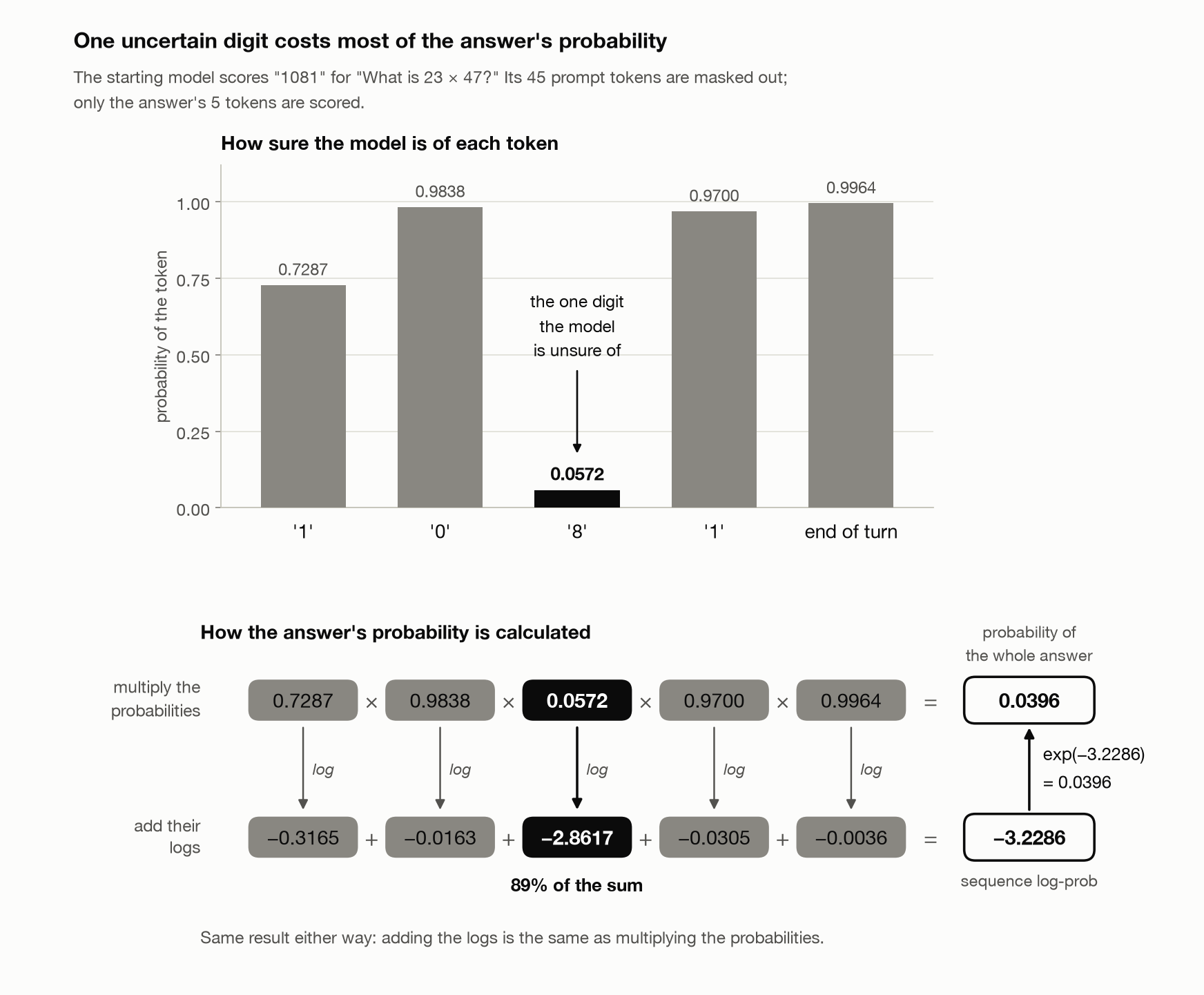
 How the model gets the probability of its answer “1081” to 23 × 47: it multiplies the probabilities of the answer’s five tokens, 0.7287 × 0.9838 × 0.0572 × 0.9700 × 0.9964 = 0.0396. Taking the log of each and adding gives the same thing as a sum, −3.2286, and exp(−3.2286) = 0.0396 takes you back. The model is nearly sure of every token except the ‘8’, whose −2.8617 is most of the sum.
Supervised fine-tuning (SFT), the kind of training posts 6 and 7 did, lowers that cross-entropy for an answer someone wrote, which raises the log-probs of its tokens. Its gradient, the signal that says which way to nudge each weight, only exists once you hand it the answer’s text: it’s the gradient of 1081’s log-prob, and without 1081 there’s nothing to differentiate.
Reinforcement learning changes where the answer comes from. The model writes its own answers, a program scores them, and training makes each answer more likely or less likely depending on how its score compares with the model’s other answers to the same question, a comparison §3 calls its advantage. It still works through each answer’s token log-probs, but weighted by that comparison, so nobody has to supply 1081, only a way to check it. The loss isn’t SFT’s cross-entropy, and it isn’t the raw sequence log-prob either. §3 derives the basic weighting, and the GRPO loss in §5 adds a clip that stops rewarding one set of sampled answers for moving a token’s probability too far, and a penalty for drifting from the starting model.
Supervised learning tells the model what to say. Reinforcement learning lets it try, checks what it said, and uses that to change what it’s likely to say next.
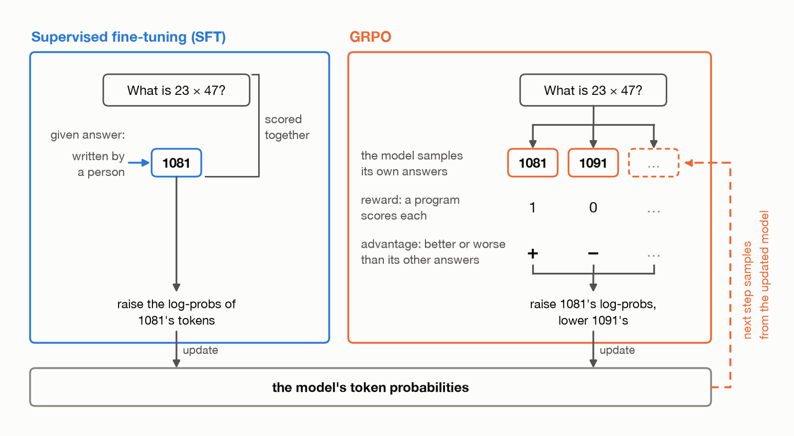
 Both methods update the same token probabilities. SFT is handed an answer someone wrote; GRPO samples its own, a program scores them, and the next samples come from the updated model.
2. A task with a checkable answer
Before training anything, there’s a question worth asking: can the model already produce correct answers, even when its first guess is wrong?
It matters because GRPO learns by comparing several answers to the same question. If the model always writes the same answer, or every answer gets the same reward, there’s little useful feedback to learn from.
I chose two-digit multiplication for this experiment. It’s simple enough to check with one line of code, but hard enough that a 0.5B model makes mistakes. That gives us both ingredients RL needs: answers the model sometimes gets right, and plenty of room to improve.
Greedy decoding and sampling
There are two ways to get an answer out of the model in this post.
Greedy decoding takes the most likely token at every step. Given the same prompt and model, it writes the same answer every time, assuming the computation itself runs the same way each time. That answer is the model’s single best guess.
Sampling draws each next token at random according to the model’s probabilities. Asking the same question eight times can give eight different answers, including ones greedy decoding would never pick.
How random the draws are is set by the temperature \(T\), and it helps to know where the model’s probabilities come from. At each step the model first gives every token in its vocabulary a raw score, a number that can be any size, positive or negative (post 1 calls these logits). A final step turns the scores into probabilities that add up to 1, and only the gaps between scores matter: the further one token’s score sits above the others, the more of the probability it takes. The temperature divides every score by \(T\) before that step, so it stretches or shrinks every gap at once:
- At \(T = 1\), the scores are left alone, and tokens are drawn from the model’s probabilities exactly as they are.
- At \(T < 1\), the gaps get wider and the probabilities get sharper, so the likely tokens are favored even more. Turned all the way down, sampling always picks the top token, which is greedy decoding.
- At \(T > 1\), the gaps get narrower and the probabilities flatter, giving unlikely tokens a better chance.
One way to picture it is a raffle, where each candidate token holds tickets in proportion to its probability and one ticket is drawn. Lowering the temperature hands more of the tickets to the favorite; raising it spreads them more evenly, so long shots win more often. The order never changes. The favorite keeps the most tickets at every temperature, and only its share moves.
Here’s what that does to a real case: §1’s question, 23 × 47, at the third digit of 1081, the one the model was unsure of. With 10 already written, these are the most likely candidates for the next token, at three temperatures, from temperature_table:
1
2
3
4
5
6
7
8
9
10
11
12
13
14
15
16
17
  Question: What is 23 x 47? Answer with just the number.
  answer so far                      "10", next is the third digit

  token             score gap  T = 0.5  T = 1.0  T = 2.0
  --------------------------------------------------------
  '3'                    0.00   0.7553   0.5118   0.2084
  '0'                   -0.63   0.2151   0.2731   0.1523
  '2'                   -1.93   0.0159   0.0742   0.0794
  '8'                   -2.19   0.0094   0.0572   0.0697
  '6'                   -3.10   0.0015   0.0230   0.0441
  all other tokens              0.0028   0.0608   0.4461

  score gap: each token's raw score minus the top token's, at T = 1.
  Each column divides every score by T, then turns them into
  probabilities. No top-k or top-p, as in the training runs.

  probability of '8' at T = 1.0, as in §1   0.0572
The T = 1.0 column is the model as it is, and it gives 8 the same 0.0572 as §1. The favorite is 3, a wrong digit, at 0.5118, and it’s the one greedy decoding would pick here. Halving the temperature to 0.5 widens every gap, so 3 goes from 0.5118 to 0.7553 and 8 falls to 0.0094. Turning the temperature down makes the right digit rarer, a small version of what this section measures: the model’s single best guess can be wrong where some of its samples are right. Doubling the temperature to 2 narrows the gaps: 3 drops to 0.2084, 8 gets 0.0697, and all the other tokens together get 0.4461, up from 0.0608.
This post uses \(T = 1\) throughout, with no top-k or top-p filtering (common tweaks that drop unlikely tokens before drawing). That keeps the answers drawn from exactly the probabilities GRPO computes later.
The temperature matters for GRPO in a second way. GRPO learns from the differences between the eight answers to a question, and a lower temperature makes those answers agree more often. When all eight come out the same, they all get the same reward, and §4 shows that a group like that teaches nothing.
How good is the model before training?
I tested the untrained model on the 200 test problems two ways: one greedy answer per problem, and eight sampled answers per problem. From the_baseline:
1
2
3
4
5
6
7
  decoding          answers  right  format-valid
  ------------------------------------------------
  greedy                200  37.5%         91.0%
  sampled, T = 1.0     1600  34.3%         86.8%

  problems right in >=1 of 8 samples 117/200 (58.5%)
    of the problems greedy gets wrong 44/125 (35.2%)
Greedy gets 37.5% right, and 91.0% of its answers are lone integers, so the instruct model mostly does as it’s told about format. Sampled answers are a little worse on both counts, 34.3% and 86.8%. That makes sense: sampling sometimes picks a less likely token instead of the most likely one.
But counting single answers misses something important. What if the model gets eight tries at each problem?
117 of the 200 problems (58.5%) were answered right in at least one of the eight samples. That share, problems with at least one right answer in eight tries, is often called pass@8. And of the 125 problems greedy gets wrong, 44 (35.2%) had a right answer somewhere among the samples.
Crossing the two problem by problem, from baseline_split:
1
2
3
4
5
6
7
  Greedy against sampling, problem by problem:

  test problems  >=1 of 8 right  none of 8 right  total
  -------------------------------------------------------
  greedy right               73                2     75
  greedy wrong               44               81    125
  total                     117               83    200
The 44 are the problems greedy gets wrong that some sample gets right. Only 2 go the other way, right when greedy and wrong in all eight samples.
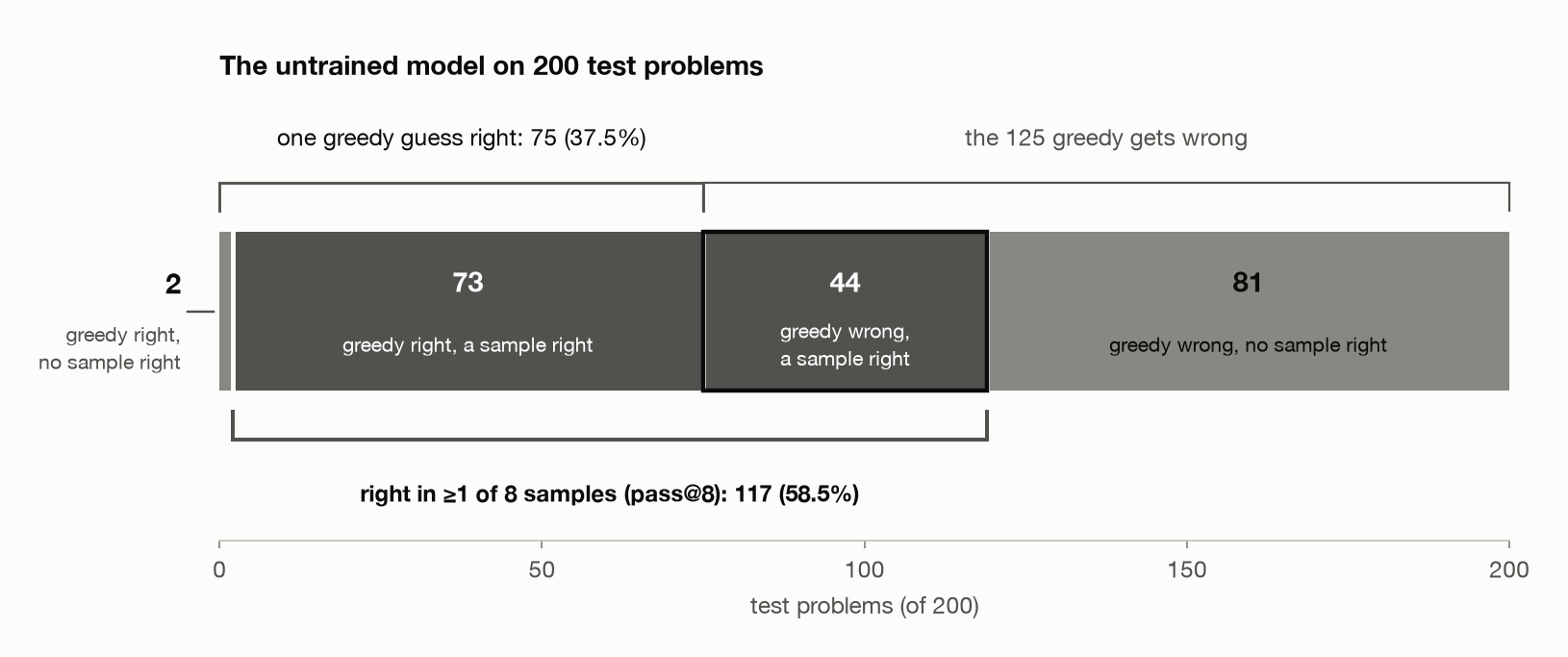
 One greedy guess gets 37.5% of the 200 test problems right; at least one of eight samples is right on 117 (58.5%). The outlined 44 are the problems greedy gets wrong that some sample gets right.
In other words, the model can sometimes write the right product even for problems its best guess gets wrong. That’s the opportunity RL can exploit. GRPO doesn’t need us to supply the right answer as a training target. It needs the model to write answers that get different rewards, so it can learn which ones to favor.
Pass@8 and greedy accuracy are different measurements, though. Greedy accuracy is one try per problem. Pass@8 is eight tries, with a program that already knows the answer picking out the right one, which nobody gets to do when the model is actually used. So the 21-point gap (58.5 minus 37.5) says there are right answers for training to reinforce. It doesn’t forecast how far greedy accuracy will rise: in §6 the three training runs gained 13.0, 21.5 and 19.5 points. And the demo doesn’t sample eight answers per problem after training, so it can’t say whether pass@8 itself moved.
The 44 tell us more than the 117. They’re the problems where the model’s default answer is wrong but a right one is within reach, and they set up a question for later: did training mostly make those 44 right, or did it also fix problems where none of the eight samples had been right? §7 splits the fixed problems along exactly that line.
There’s an important limitation, though. If all eight answers to a problem are wrong, they all get a reward of 0. Each one scores exactly the average of the eight, and since GRPO compares each answer with that average, the group gives no learning signal. The same happens if all eight are right. §4 counts how often that happens.
This doesn’t mean RL can never learn a problem it starts out getting wrong. An update changes weights that every problem shares, so it can carry over to other problems, and later samples may find right answers earlier ones missed. The 200 test problems are never trained on at all, so anything that changes on them, the 44 included, changes through that sharing. But without variation in rewards, GRPO has nothing useful to learn from that particular group.
DeepSeekMath’s authors saw a related limit at scale: RL improved how often the most common answer among \(K\) samples was right, a majority vote, but not how often at least one of the \(K\) samples was (Shao et al., Figure 7). My reading of that is that RL can help a model get a problem right more often when some of its tries already got it right. It doesn’t necessarily help with problems that none of its tries got right before.
Correct arithmetic isn’t always a correct answer
One more detail before training: the reward checks both the number and the format the prompt asked for.
The prompt asks for just the number, but some sampled answers aren’t. The first three, one per problem, from the_baseline:
1
2
3
4
  Sampled answers not a lone integer, first three, one per problem:
    "35 x 11 = 385"
    "3, 854"
    "26 x 83 = 2118"
The first has the right product inside a sentence, the second splits a number with a comma and a space, and the third is a sentence with the wrong product: 26 × 83 is 2158. All three score 0, the same as a wrong number, because the program checks the format as strictly as the number.
That strictness raises a question for later: when accuracy goes up after training, is the model getting better at multiplication, or just at answering in the right format? We’ll come back to that in §7, and to 35 × 11 and 26 × 83 with it.
The model knows how to produce more correct answers than it reliably chooses. GRPO gives us a way to turn some of those occasional successes into more consistent behavior.
3. From rewards to a gradient
In SFT we already know which answer we want, and training raises its log-prob. RL starts somewhere else. Nobody hands the model the answer: it writes its own, and a reward scores each one. So SFT tells the model which answer to make more likely, and RL uses the reward to decide whether an answer the model wrote should become more likely or less. This section turns that score into an update, and it needs a little vocabulary first.
In RL terms, the model is the policy: the rule that picks what to do. For a language model the policy gives a probability to each next token, and multiplying those together gives the probability of a whole answer (§1’s sum, in log-probs). Here a whole answer counts as one action: the model gets a multiplication question, writes an answer, and the reward is the score that answer gets, 1 if it’s right and 0 if not. In general a policy can collect rewards over many steps, and the total is called the return; here there’s one reward per answer, at the end, so the return is just that reward. The symbols:
| symbol | means | here |
|---|---|---|
| \(\theta\) | the trainable weights | the LoRA adapters’ weights |
| \(q\) | a question | “What is 23 × 47? …” |
| \(o\) | one answer the model wrote (its output) | 1081 and the end-of-turn token |
| \(\pi_\theta(o \mid q)\) | the probability the policy gives answer \(o\) to question \(q\) | 0.0396 for 1081 |
| \(\log \pi_\theta(o \mid q)\) | that answer’s sequence log-prob, §1’s sum | −3.2286 |
| \(r\) | the reward the answer got | 1 or 0 |
| \(b\) | a baseline: a reference score to compare \(r\) against, chosen without looking at which answer was written | how well the model usually does on \(q\); §4 estimates it from a group of answers |
| \(\alpha\) | the learning rate, how big each nudge is | |
| \(\nabla_\theta\) | the gradient with respect to the weights: which way to nudge each one to raise what follows |
The update that comes out is due to Williams (1992), who called it REINFORCE, an acronym he spells out as “REward Increment = Nonnegative Factor times Offset Reinforcement times Characteristic Eligibility”. In the notation used today:
\[\Delta\theta = \alpha\,(r - b)\,\nabla_\theta \log \pi_\theta(o \mid q)\]This is the update from one answer. In training it’s averaged over many: §4 samples eight answers per question and §6 uses eight questions per step, so each step averages 64 of these. Read it right to left, one piece at a time.
\(\nabla_\theta \log \pi_\theta(o \mid q)\) says what to change. It’s exactly the direction SFT would step in if someone had handed it \(o\) as the answer: the direction that makes \(o\) more likely. The difference from SFT is that the model wrote \(o\) itself.
Here’s SFT’s update in the same notation. Call the answer someone wrote \(o^*\) (
\[\Delta\theta = \frac{\alpha}{\lvert o^* \rvert}\,\nabla_\theta \log \pi_\theta(o^* \mid q)\]1081in §1) and its number of tokens \(\lvert o^* \rvert\) (five there, the end-of-turn token included). SFT’s loss is §1’s cross-entropy, the mean of the negative token log-probs, which is the sequence log-prob turned around and divided by the token count: \(-\log \pi_\theta(o^* \mid q) \,/\, \lvert o^* \rvert\). Training lowers a loss by stepping against its gradient, so SFT’s update isSet beside REINFORCE, \(o^*\) takes the place of \(o\) and there’s no \(r - b\), so every target answer is made more likely. For one answer, dividing by \(\lvert o^* \rvert\) only shrinks the step. Across a batch it also gives each token of a short answer more weight than each token of a long one.
- \(r - b\) says which way to step, and how far. This difference, how much better the answer did than expected, is called its advantage. An answer that scored above the baseline has a positive advantage and is made more likely, in proportion to how far above; an answer below it has a negative advantage and is made less likely.
- \(\alpha\) sets the size of the step.
The reward says whether an answer was good, the log-prob gradient says how to make that answer more or less likely, and the advantage connects the two. With \(r - b = 1\) for every answer, this would be SFT on the model’s own answers.
Why it points uphill. What we want is a high average reward. Write \(\mathbb{E}_{o \sim \pi_\theta}[\,r\,]\) for the average reward over the answers the policy might write to \(q\), each weighted by its probability. The verifier, the program that checks the answer, has no gradient: it can say 1081 is right, but not how to change any LoRA weight to make right answers likelier. The probabilities do have one, and that’s enough, because of the policy-gradient identity:
To see where it comes from, start on the left and write \(r(o)\) for the reward of answer \(o\).
Write the average as a sum. The average reward adds up the reward of every answer the model could write, each weighted by its probability:
\[\mathbb{E}_{o \sim \pi_\theta}[\,r\,] = \sum_o \pi_\theta(o \mid q)\, r(o)\]Take the gradient inside the sum. The reward doesn’t depend on \(\theta\), since the verifier only checks the answer, so the gradient touches only the probabilities:
\[\nabla_\theta\, \mathbb{E}_{o \sim \pi_\theta}[\,r\,] = \sum_o r(o)\, \nabla_\theta \pi_\theta(o \mid q)\]This is the line we can’t compute: it needs every answer the model could possibly write.
Use the derivative of the log. The derivative of a log is the derivative of the value divided by the value, \(\nabla_\theta \log \pi_\theta = \nabla_\theta \pi_\theta \,/\, \pi_\theta\). Multiplying both sides by \(\pi_\theta\) gives
\[\nabla_\theta \pi_\theta(o \mid q) = \pi_\theta(o \mid q)\,\nabla_\theta \log \pi_\theta(o \mid q)\]Substitute. Putting that in place of \(\nabla_\theta \pi_\theta\) in step 2 brings the probability back into the sum:
\[\nabla_\theta\, \mathbb{E}_{o \sim \pi_\theta}[\,r\,] = \sum_o \pi_\theta(o \mid q)\, r(o)\, \nabla_\theta \log \pi_\theta(o \mid q)\]Read it as an average again. Each term is weighted by its probability, as in step 1, so the sum is an average over the answers the policy writes. That’s the right side of the identity:
\[\sum_o \pi_\theta(o \mid q)\, r(o)\, \nabla_\theta \log \pi_\theta(o \mid q) = \mathbb{E}_{o \sim \pi_\theta}\big[\,r\,\nabla_\theta \log \pi_\theta(o \mid q)\,\big]\]An average can be estimated by sampling answers and averaging them, with no need to list every possible one, and that’s what training does with its 64 answers per step.
On the left is the direction that raises the average reward, which step 2 showed we can’t compute directly. On the right is the average of something we can compute for one sampled answer: its reward times the gradient of its log-prob. The reward never needs a gradient of its own. The gradient comes from the model’s log-prob, and the verifier only supplies the weight. The baseline argument below uses steps 2 to 5 in reverse.
What Williams proved, and what he didn’t. His Theorem 1 says that, on average over the answers the policy might write, this update is \(\alpha\) times the gradient of the expected reward. So each update is a noisy estimate of the direction that raises the average score, and in his words, \((r - b)\,\nabla_\theta \log \pi_\theta\) “represents an unbiased estimate”. Only the average is promised; a single update can still point the wrong way. The condition is that the baseline is “conditionally independent of” the action, which is why \(b\) mustn’t depend on which answer was written. When it doesn’t, its part of the update averages to zero, because the probabilities of all the possible answers always add up to 1:
\[\mathbb{E}_{o \sim \pi_\theta}\big[\,b\,\nabla_\theta \log \pi_\theta(o \mid q)\,\big] = b \sum_o \nabla_\theta \pi_\theta(o \mid q) = b\,\nabla_\theta 1 = 0\]Any such baseline keeps the estimate unbiased, including \(b = 0\), and Williams says plainly that his results “offer no basis for comparing various choices of reinforcement baseline”.
So why have one? Take a question the model gets right 80% of the time. With \(b = 0\):
| answer | \(r\) | advantage \(r - b\) |
|---|---|---|
| right | 1 | +1 |
| wrong | 0 | 0 |
A wrong answer gets no update at all; only right answers move, always up. A question the model already gets right every time still pushes all its answers up, though there’s nothing left to learn. Now set \(b\) to how well the model usually does on that question, \(b = 0.8\):
| answer | \(r\) | advantage \(r - b\) |
|---|---|---|
| right | 1 | +0.2 |
| wrong | 0 | −0.8 |
A right answer is still pushed up, but only a little, because it’s what the model does most of the time anyway. A wrong answer is pushed down hard, because it did much worse than expected. On a hard question with \(b = 0.2\) it flips: a rare right answer gets +0.8 and a wrong one −0.2. So a right answer to a hard question counts for a lot and a right answer to an easy one for little. A baseline like this also tends to make each noisy step less noisy. In Sutton and Barto’s words (§13.4), “the baseline leaves the expected value of the update unchanged, but it can have a large effect on its variance”. Williams proves the first half of that sentence, not the second.
From REINFORCE to PPO and GRPO. Two practical questions are left. Where does \(b\) come from, when “how well the model usually does on this question” isn’t something we can look up? And what stops one step from making a sampled answer far likelier than it should be? The update in the paper that introduced PPO (Proximal Policy Optimization, Schulman et al., Equation 1), the method most language-model RL used before GRPO, is this one with an estimated advantage \(\hat A\) in place of \(r - b\). §4 is about where that estimate comes from: PPO’s answer is a second network, and GRPO’s is to ask the same question several times and compare the rewards. §5 is about the second question.
4. Groups instead of a value model
The baseline should be “how well the model usually does on this question”. Getting that number is the expensive part.
PPO gets that number from a second network. GRPO gets it by asking the same question several times and averaging the rewards, which saves training a second model. The catch is that GRPO only learns from groups whose answers got different rewards, and with the demo’s eight answers per question, 61.1% of groups didn’t.
Two ways to get a baseline
PPO’s answer: a second network. PPO, which RLHF also uses (§8), trains a value model: a second network that reads the question and the answer so far and predicts the reward to come. Its prediction is the baseline. That means training and holding a second large model next to the first, which DeepSeekMath’s authors call “a substantial memory and computational burden” (Shao et al., §4.1.1).
GRPO’s answer: ask the question several times. GRPO (Group Relative Policy Optimization) was introduced in the same DeepSeekMath paper. Instead of predicting how well the model usually does on a question, it measures it: sample a group of \(G\) answers to the same question, score them all, and use the group’s own average as the baseline. Each answer’s advantage is its reward compared with the rest of its group, divided by the group’s spread (§4.1.2 of the paper). With \(r_i\) the reward of answer \(i\), and std the standard deviation, a measure of how spread out the rewards are:
\[\hat A_i = \frac{r_i - \operatorname{mean}(r_1, \ldots, r_G)}{\operatorname{std}(r_1, \ldots, r_G) + 0.0001}\]The demo uses the sample standard deviation, which divides by \(G - 1\) rather than \(G\). The 0.0001 isn’t in the paper’s formula. It’s there so a group whose rewards are all equal divides by something other than zero. Every token of answer \(i\) shares the one advantage \(\hat A_i\). In group_advantages, with one row per group:
1
2
3
    mean = rewards.mean(dim=1, keepdim=True)
    std = rewards.std(dim=1, keepdim=True)
    return (rewards - mean) / (std + eps)
One thing to keep straight about history: DeepSeekMath introduced GRPO with a learned reward model doing the scoring, a network trained to score answers (§8). Scoring with a program that checks the answer came later. DeepSeek’s Prover-V1.5 trained with GRPO on a proof checker’s verdict, “a reward of 1 if verified as correct, and 0 otherwise” (§2.3), and DeepSeek-R1 scored math, code and logic with rules (§2.2). That’s the version this demo builds.
Three groups of eight answers
The demo first estimated each training question’s pass rate, the share of its sampled answers that are right, then picked the question with the lowest, the one nearest 50%, and the highest, and sampled a group of eight answers to each. From groups_and_advantages, the hardest:
1
2
3
4
5
6
7
8
9
10
11
12
  31 x 51 = 1581   (pass rate estimate 0.00)
  #  response  reward  advantage
  --------------------------------
  1    "1641"       0     +0.000
  2    "1501"       0     +0.000
  3    "1601"       0     +0.000
  4    "1601"       0     +0.000
  5    "1661"       0     +0.000
  6    "1591"       0     +0.000
  7    "1691"       0     +0.000
  8    "1661"       0     +0.000
  mean 0.000   std 0.000   (r - mean) / (std + 0.0001)
Every answer is a near miss, all eight score 0, the mean is 0 and so is the spread, and every advantage is exactly zero. The middle question, also from groups_and_advantages:
1
2
3
4
5
6
7
8
9
10
11
12
  46 x 32 = 1472   (pass rate estimate 0.50)
  #    response  reward  advantage
  ----------------------------------
  1  "New York"       0     -0.935
  2      "1352"       0     -0.935
  3      "1472"       1     +0.935
  4      "1452"       0     -0.935
  5      "1472"       1     +0.935
  6      "1452"       0     -0.935
  7      "1472"       1     +0.935
  8      "1472"       1     +0.935
  mean 0.500   std 0.535   (r - mean) / (std + 0.0001)
Four right, four wrong. The mean is 0.500, the sample standard deviation is 0.535, and each answer’s advantage is ±0.935: the four 1472s are pushed up by the same amount the four wrong answers are pushed down. New York gets the same −0.935 as 1452. The reward is 0 for both, and the advantage can’t tell a near miss from nonsense. And the easiest, from the same groups_and_advantages:
1
2
3
4
5
6
7
8
9
10
11
12
  12 x 24 = 288   (pass rate estimate 1.00)
  #  response  reward  advantage
  --------------------------------
  1     "288"       1     +0.000
  2     "288"       1     +0.000
  3     "288"       1     +0.000
  4     "288"       1     +0.000
  5     "288"       1     +0.000
  6     "288"       1     +0.000
  7     "288"       1     +0.000
  8     "288"       1     +0.000
  mean 1.000   std 0.000   (r - mean) / (std + 0.0001)
All eight right, and all zero again. A question that’s always right and a question that’s never right both teach the model nothing. In both, every answer is exactly as good as the group’s average, so there’s nothing to prefer. GRPO can only learn the distinctions the reward makes, and only from groups where the rewards differ.
How often does a group teach nothing?
For the 256 training questions, the demo sampled 16 answers each:
1
2
3
4
5
  Pass rates of the 256 train questions (16 samples each):
    never right                      97
    always right                     25
    in between                       134
    mean pass rate                   0.326
97 questions were never answered right in 16 tries and 25 always were: 122 of the 256 in all, against 134 in between. A group of answers to one of those questions will almost always be all-equal. Then, cutting another 16 fresh samples per question into groups of different sizes and counting the groups whose rewards are all equal, from groups_and_advantages:
1
2
3
4
5
6
7
8
9
10
11
  G   groups  measured  analytic
  --------------------------------
  2     2048     0.854     0.856
  4     1024     0.733     0.738
  8      512     0.611     0.635
  16     256     0.492     0.553

  measured: 16 fresh samples per question, cut into groups of G.
  analytic: mean over questions of p^G + (1-p)^G, with each p
  estimated from 16 other samples. p^G + (1-p)^G is convex in p,
  so plugging in an estimated p overstates it (Jensen's inequality).
With the demo’s \(G = 8\), 61.1% of groups carry no signal, and only 38.9% have both a right and a wrong answer in them (the mixed column of the table below). Even with 16 answers per question, 49.2% of groups carry none.
The measured column counts real groups. The analytic column is what you’d predict from the pass rates alone: if a question is right with probability \(p\) and the \(G\) answers are independent, all \(G\) are right with probability \(p^G\) and all wrong with probability \((1-p)^G\), so the group is all-equal with probability \(p^G + (1-p)^G\), averaged over the questions. It overshoots a little, more for bigger \(G\). Each \(p\) is itself estimated from 16 samples, and because \(p^G + (1-p)^G\) curves upward on both sides for any \(G\) of 2 or more, an estimate that’s wrong in either direction raises it on average. That’s Jensen’s inequality, and it says the prediction should come out too high on average, which is what the table shows. It doesn’t account for the exact gaps: the measured column is itself a count over a few hundred groups, 512 at \(G = 8\) and 256 at \(G = 16\), with noise of its own.
Choosing a group size
Bigger groups help: a question with a pass rate of 20% gives an all-equal group of two with probability \(0.2^2 + 0.8^2 = 0.68\), and an all-equal group of eight with only \(0.2^8 + 0.8^8 \approx 0.168\). But each answer costs a full generation, and which group size is the better buy depends on what you count. The same measured groups, counted two ways, from groups_and_advantages:
1
2
3
4
5
6
7
8
9
  G   mixed  mixed groups per 1,000 answers
  -------------------------------------------
  2   14.6%                              73
  4   26.7%                              67
  8   38.9%                              49
  16  50.8%                              32

  mixed: 1 - measured, groups with both a right and a wrong answer.
  mixed groups per 1,000 answers: (1000 / G) x mixed.
A mixed group has both a right and a wrong answer in it. Per 1,000 generated answers, groups of two give 73 mixed groups and groups of sixteen give 32, so small groups cover more questions that teach something. Counted by answers it goes the other way: in a mixed group every answer’s reward differs from the mean, so every answer gets a nonzero advantage, and the share of answers that carry signal is the mixed column, 14.6% at \(G = 2\) and 50.8% at \(G = 16\). Neither count says how useful each gradient is. What they do show is that group size trades how many questions get a signal against how many answers get one.
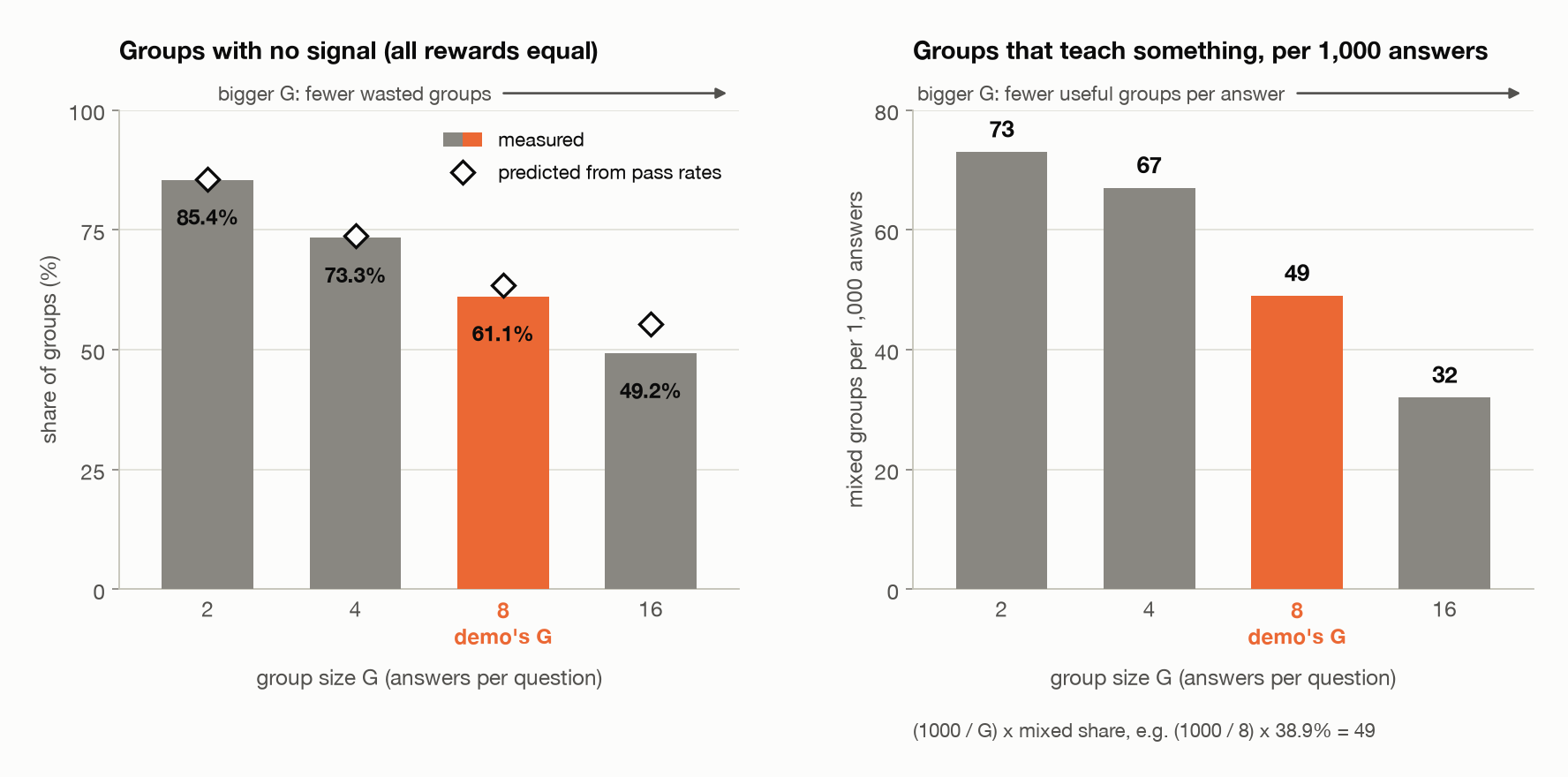
 Left: the share of groups whose answers all got the same reward, so every advantage is zero (bars measured on 16 fresh samples per question; diamonds predicted from each question’s estimated pass rate). Right: the same groups, counted as mixed groups per 1,000 answers generated. Bigger groups waste fewer questions but spend more answers on each group that teaches something.
DAPO and Dr. GRPO
The field has two responses to this, both with a direct line to these tables. DAPO (§3.2) uses dynamic sampling: it filters out groups whose answers are all right or all wrong and keeps sampling until a batch is full of groups that teach something, because “A zero advantage results in zero policy gradients”.
Dr. GRPO (§3.1) points at the division by the standard deviation. A group with one right answer in eight has a small spread, so dividing by it makes that one answer’s advantage large. Questions that are nearly always right or nearly always wrong get weighted more than questions in the middle, a difficulty bias, and Dr. GRPO drops the division (§3.2). This demo keeps it, to match DeepSeekMath. DAPO is about getting groups that teach something, and Dr. GRPO about how much each one counts once you have it.
Is the group’s average a fair baseline?
The group’s average also isn’t quite the baseline of §3. Williams’s guarantee needs a baseline chosen without looking at which answer was written, and the group’s average includes answer \(i\)’s own reward. Without the division, that costs only a rescaling. Some algebra on the mean gives
\[r_i - \operatorname{mean}(r_1, \ldots, r_G) = \frac{G-1}{G}\Big(r_i - \operatorname{mean}(\text{the other } G-1 \text{ rewards})\Big)\]and the other answers were sampled independently of answer \(i\), so their average is a fair baseline for it. The step is the unbiased one shrunk by \(\tfrac{G-1}{G}\), which is \(\tfrac{7}{8}\) at \(G = 8\). The standard deviation depends on \(r_i\) as well, and once you divide by it Williams’s theorem no longer covers the update. That’s the part Dr. GRPO objects to.
So GRPO does away with the value model, but it swaps in a new dependency: the model has to write answers that get different rewards.
5. One update by hand
§4 was about where the learning signal comes from: each answer’s advantage says which way to push it, and how hard. This section is about turning that signal into an update without pushing the model too far in one go, the second question §3 left open. With advantages in hand, the update is the REINFORCE step of §3: raise the log-prob of answers with a positive advantage and lower it for answers with a negative one. GRPO adds two safety features from PPO to that step, a clipped probability ratio and a KL penalty (a cost for drifting too far from the starting model), both meant to limit how far the policy moves. This section explains both, then takes one group, the 46 × 32 group from §4, and runs two gradient steps on it by hand.
The hand-run shows how far one update can go. One gradient step on that group left one token about a ten-thousandth as likely as when the model wrote it, even though the clip stops rewarding any push that takes a token more than 20% above or below the probability it was sampled with, and on the next step the KL penalty made up almost all of the loss. The clip caps what a token earns for moving, and puts no limit on how far it moves.
The probability ratio and the clip
Sampling is the slow part, so PPO and GRPO allow several gradient steps, called inner steps, on the same batch of sampled answers. After the first step, though, the policy being trained is no longer the one that wrote the answers. The probability ratio tracks how far it’s moved, token by token: the probability the current policy gives a token, divided by the probability the policy that sampled it gave it. A ratio of 1 means no change, 1.2 means the token is 20% more likely than when it was sampled, and 0.5 means half as likely. On the first inner step it’s exactly 1 everywhere, because the two policies are the same.
PPO’s objective (Equation 7 of the PPO paper) takes the smaller of two terms: the ratio times the advantage, and the same with the ratio clipped to the range \(1 - \epsilon\) to \(1 + \epsilon\), “say, ϵ = 0.2”. The demo uses 0.2 too, so the range is 0.8 to 1.2. For a right answer, with a positive advantage, the objective wants its tokens more likely, but once a token’s ratio is past 1.2 the clipped term wins, it’s constant, and that token stops contributing to the gradient. For a wrong answer the boundary is 0.8: once a token is less than 0.8 times as likely, pushing it further down earns nothing. So the clip takes away the incentive to go further, but it doesn’t stop a token from going further. Every token shares the same weights, and an update aimed at other tokens can still carry this one past 1.2 or below 0.8. The paper calls the result “a lower bound (i.e., a pessimistic bound)” on the unclipped objective. It bounds the objective, and not how far the policy can move.
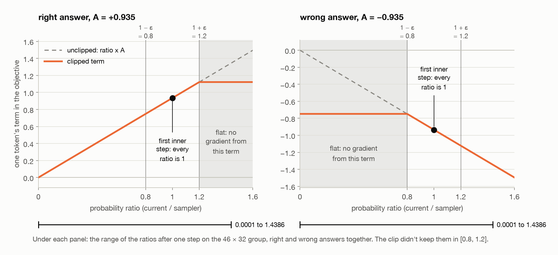
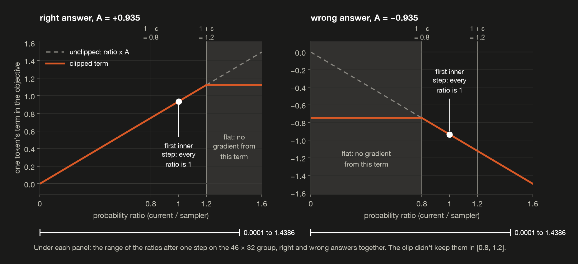 One token’s term in PPO’s clipped objective against its probability ratio, with A the answer’s advantage in §4’s group for 46 × 32. For the right answer the line goes flat past 1.2, and for the wrong one below 0.8, so going further earns nothing. Nothing stops a token getting there, though: one step on this group put the ratios between 0.0001 and 1.4386 (the step 2 row of the receipt in “Two inner steps on one group” below).
The KL penalty
Chasing a reward can pull the policy a long way from the model it started as, toward outputs that happen to score well without being what we wanted (§8 calls this reward hacking). The reward only checks the final answer and its format, the right number written as a lone integer, so nothing in it protects anything else the starting model could do. The KL penalty works like a leash back to the starting model, which is kept frozen and called the reference model. The further the policy’s probabilities drift from the reference’s, the more the loss charges.
How far the policy has drifted is measured with KL divergence (KL for Kullback-Leibler), a measure of how different two probability distributions are: it’s zero when they’re identical and grows as they drift apart. For one question, the KL divergence of the policy from the reference goes through every answer the policy could write, takes the log of how much likelier the policy makes that answer than the reference does, and averages those logs, weighting each answer by how likely the policy is to write it. Write \(o\) for any one answer, and \(\pi_\theta(o)\) and \(\pi_{\text{ref}}(o)\) for the probability the policy and the reference give the whole answer (§3’s \(\pi_\theta(o \mid q)\), with the question left out to keep the formula short), whose log is §1’s sequence log-prob. Then
\[D_{KL}\big(\pi_\theta \,\Vert\, \pi_{\text{ref}}\big) = \sum_{o} \pi_\theta(o)\,\log\frac{\pi_\theta(o)}{\pi_{\text{ref}}(o)}\]The order matters, because KL divergence isn’t symmetric: this one weights by the policy’s probabilities, so it’s an average over the answers the policy itself writes. The sum runs over every answer the model could write, far too many to add up, so GRPO estimates it from the answers it samples and subtracts that estimate from what training maximizes, scaled by a weight \(\beta\) that sets how hard the leash pulls. Training then raises the reward while paying for its distance from the reference, a trade §8 writes out as a formula for RLHF. Where that penalty goes differs by method. PPO as used for RLHF subtracts it from the reward, token by token (§8); GRPO, in DeepSeekMath’s words, “instead of adding KL penalty in the reward, GRPO regularizes by directly adding the KL … to the loss”.
Because an answer’s log-prob is the sum of its tokens’ log-probs (§1), the log in that formula splits into one piece per token, and the estimate works token by token. For each token it asks one question: how much likelier, or less likely, does the policy make this token than the reference does? That’s a probability ratio again, policy over reference this time instead of policy over sampler. A token left at a ratio of 1 costs nothing. Moving it either way costs something, but the charge is lopsided: the cost of pushing a token down grows much faster than the cost of pushing one up.
In symbols, the estimate is the one Schulman’s note on approximating KL divergence calls \(k_3\). Per token, write \(d\) for the reference model’s log-prob of the token minus the policy’s. Then the estimate is \(e^{d} - d - 1\). Here \(e^{d}\) is the reference’s probability over the policy’s, one over the ratio, and that’s where the lopsidedness comes from. Push a token down and \(e^{d}\) grows without limit; push it up and \(e^{d}\) shrinks toward zero, leaving only \(-d\), which grows slowly. The estimate is zero when the two agree (\(d = 0\)), and never negative, since \(e^{d} \ge 1 + d\) for any \(d\); Schulman’s note shows that, for tokens sampled from the policy, its average is the true KL divergence of the policy from the reference. The hand-run’s receipts below call this quantity r; in this post \(r\) is the reward, so I’ve written it as \(d\). DeepSeekMath uses this estimator too (its Equation 4), and the demo runs DeepSeekMath’s \(\beta = 0.04\).
Here’s the charge at a few ratios, in mirror pairs, from kl_estimate, the same expression the training loss uses, printed by uv run demo08 --kl-table (d08_kl_table.py):
1
2
3
4
5
6
7
8
9
10
11
12
13
14
15
16
17
18
19
20
21
22
23
24
  ratio = policy probability / reference probability of a token;
  d = reference log-prob - policy log-prob = -ln(ratio);
  estimate = exp(d) - d - 1, as in demo 08's training loss.

  ratio   as a number        d   estimate
  -----------------------------------------
  x10         10.0000  -2.3026     1.4026
  x2           2.0000  -0.6931     0.1931
  x1.5         1.5000  -0.4055     0.0721
  x1           1.0000  +0.0000     0.0000
  /1.5         0.6667  +0.4055     0.0945
  /2           0.5000  +0.6931     0.3069
  /10          0.1000  +2.3026     6.6974
  /100         0.0100  +4.6052    94.3948
  /10000     1.00e-04  +9.2103  9989.7897

  Mirror pairs, same factor either way:

  pair        more likely  less likely
  --------------------------------------
  x2 vs /2         0.1931       0.3069
  x10 vs /10       1.4026       6.6974

  Each row is one token's estimate, not the KL divergence itself.
Read it in pairs. A token the policy makes twice as likely as the reference does costs 0.1931, and one it makes half as likely costs 0.3069. At ten times either way it’s 1.4026 against 6.6974, and a token made ten thousand times less likely costs 9989.7897. That lopsidedness is in the charge for one sampled token. The KL divergence itself is an average over the tokens the policy writes, and a token the policy has made rare is one it rarely writes, so in a fresh sample its large charge is rarely counted. Step 2 of the hand-run below counts one anyway, because it rescores answers written before the push.
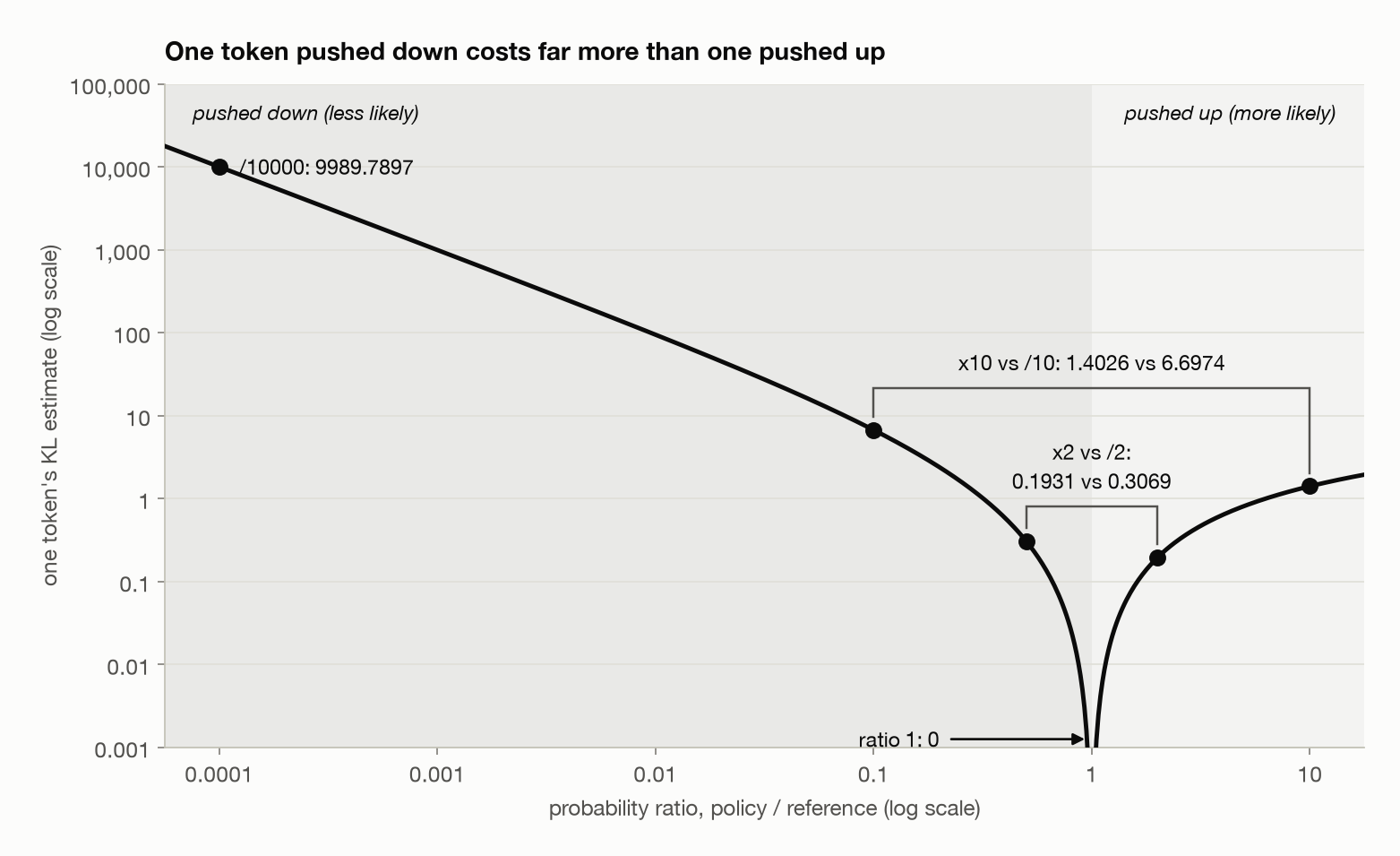
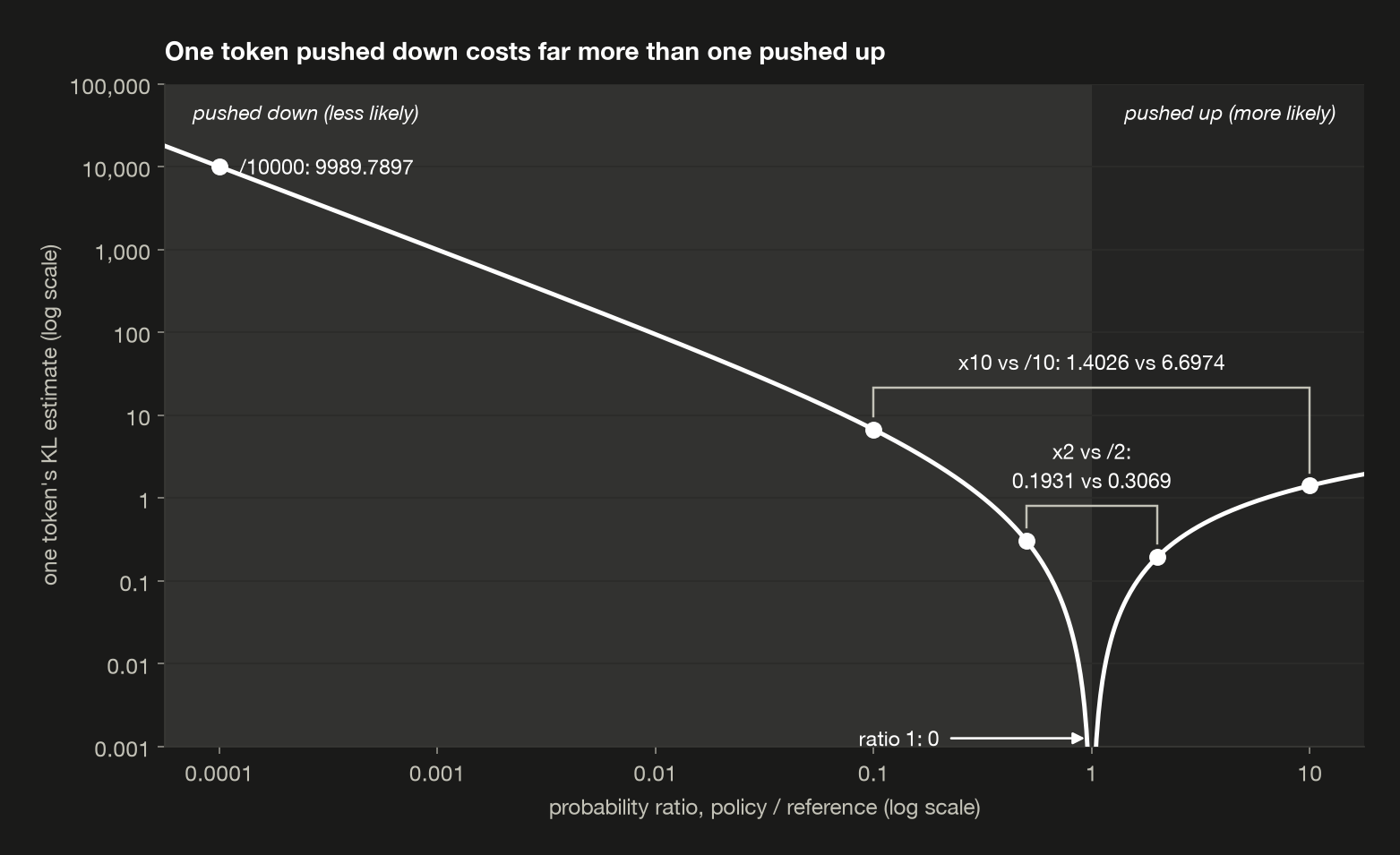 The KL estimate for one token against how much likelier the policy makes it than the reference. The same factor costs more downward than upward: 0.1931 for twice as likely and 0.3069 for half, 1.4026 for ten times and 6.6974 for a tenth.
The demo’s reference model costs no extra memory. The policy is Qwen plus LoRA adapters, and the reference is the same network with the adapters’ contribution multiplied by zero, which is the starting model bit for bit (adapters_off). That’s one reason a 0.5B model and its reference fit on a laptop.
The clip and the KL penalty both hold the policy back, but they measure it against different models:
| the clip | the KL penalty | |
|---|---|---|
| compares the policy with | the policy that sampled the current answers | the frozen reference |
| what it pushes against | a token earning more for moving, over the steps on one batch | the whole run drifting from the starting model, charged in the loss but never capped |
| over training | its yardstick is replaced with every new batch | its yardstick never changes |
In the hand-run below the two start out as the same model, because fresh adapters make the sampler the starting model too.
The GRPO objective
The symbols, for answer \(i\) of a group and its token \(t\):
| symbol | means |
|---|---|
| \(G\) | answers per group, 8 |
| \(o_i\), \(\lvert o_i \rvert\) | answer \(i\), and its number of tokens, the end-of-turn token included |
| \(\pi_\theta\), \(\pi_{\text{old}}\), \(\pi_{\text{ref}}\) | the policy being trained, the policy that sampled the answers, the frozen reference |
| \(\rho_{i,t}\) | the probability ratio of token \(t\): \(\pi_\theta\)’s probability for it divided by \(\pi_{\text{old}}\)’s |
| \(\hat A_i\) | answer \(i\)’s advantage, from §4, shared by all its tokens |
| \(\epsilon\) | the clip range, 0.2 |
| \(d_{i,t}\) | \(\log \pi_{\text{ref}} - \log \pi_\theta\) for token \(t\) |
| \(\beta\) | the weight on the KL term, 0.04 |
The demo maximizes DeepSeekMath’s Equation 3, written in these symbols:
\[\mathcal{J}(\theta) = \frac{1}{G}\sum_{i=1}^{G}\frac{1}{\lvert o_i\rvert}\sum_{t=1}^{\lvert o_i\rvert}\Big(\min\big[\rho_{i,t}\hat A_i,\ \operatorname{clip}(\rho_{i,t}, 1-\epsilon, 1+\epsilon)\,\hat A_i\big] - \beta\,\big(e^{d_{i,t}} - d_{i,t} - 1\big)\Big)\]From the inside out: each token gets its clipped term minus its KL penalty; those are averaged over the answer’s tokens; the answers’ averages are averaged over the group. The loss is \(-\mathcal{J}\). In code, the core of grpo_objective, whose inputs are each token’s log-prob under the three policies:
1
2
3
4
5
6
7
8
    adv = advantages.unsqueeze(1)
    ratio = torch.exp(logp - old_logp)
    clipped_ratio = ratio.clamp(1 - clip, 1 + clip)
    surrogate = torch.minimum(ratio * adv, clipped_ratio * adv)
    log_ref_ratio = ref_logp - logp
    kl = torch.exp(log_ref_ratio) - log_ref_ratio - 1
    per_answer = masked_mean(surrogate - beta * kl, mask)
    loss = -per_answer.mean()
The clipped term is called the surrogate, because it stands in for the expected reward: its gradient is the policy-gradient step, but it isn’t the reward itself.
Other papers write GRPO differently. DeepSeek-R1 computes one ratio per answer rather than per token (§2.1, Equation 1), and DAPO and Dr. GRPO change the averaging and drop the KL term. The formula above is the one this demo runs.
Two inner steps on one group
Here are two inner steps on the 46 × 32 group, from one_update, starting from fresh adapters, whose \(B\) matrix starts at zero, as in post 6, so the policy is exactly the starting model. Each row is measured as its step begins, before the optimizer changes any weights, so step 1’s row is the starting model and step 2’s row is the model after one update:
1
2
3
4
5
6
7
8
9
10
11
12
13
14
  The group for 46 x 32 from post §4, adapters fresh, lr 3e-05.
  2 gradient steps on the same 8 answers (GRPO's inner steps).

  step  ratio min  ratio max  clipped  surrogate         KL      loss
  ---------------------------------------------------------------------
  1        1.0000     1.0000     0.0%    +0.0000  -1.44e-08   +0.0000
  2        0.0001     1.4386    28.9%    +0.0580   4.52e+02  +18.0031

  Step 1: the policy is the sampler, so every ratio is exactly 1, and
  the adapters start at zero, so the KL is 0 (to float rounding).
  Step 2 scores the same answers again. Where a token's log-prob fell
  below the reference's, the KL term exp(r) - r - 1, r = ref - logp,
  grows exponentially in r; where a ratio crossed the clip in the
  advantage's direction, that token's surrogate gradient is zero.
Step 1 is the clean case. The policy is the sampler, so every ratio is exactly 1, nothing is clipped, and the policy is also the reference, so the KL is zero (the −1.44e-08 is float rounding). The surrogate’s value is zero too, because the advantages of a group always add up to zero. Its gradient isn’t zero, though. At a ratio of 1, the gradient of \(\rho_{i,t}\) is the gradient of the token’s log-prob, \(\log \pi_\theta(o_{i,t})\), and the KL term’s gradient is zero at \(d = 0\), so the step-1 gradient is
\[\nabla_\theta \mathcal{J} = \frac{1}{G}\sum_{i=1}^{G}\frac{\hat A_i}{\lvert o_i\rvert}\sum_{t=1}^{\lvert o_i\rvert}\nabla_\theta \log \pi_\theta(o_{i,t})\]That’s §3’s REINFORCE step, with the group’s advantages as weights and each answer’s tokens averaged. The advantages cancel in the value, but the gradients don’t, because the right and wrong answers are different tokens with different gradients. A loss of zero doesn’t mean there’s nothing to learn.
The second step, on reused answers
Step 2 reuses the same eight answers, and shows why PPO-style methods need their safety features. One step at this learning rate moved some tokens a long way. The smallest ratio is 0.0001: some token now has about a ten-thousandth of the probability it had when it was sampled. The largest is 1.4386, a token about 44% more likely than when it was sampled. It’s past the clip’s 1.2 after a single step. 28.9% of answer tokens are past the clip in their advantage’s direction (above 1.2 in a right answer, below 0.8 in a wrong one), and contribute no gradient from the surrogate.
The KL estimate has gone from zero to 4.52e+02. That’s the per-token estimates averaged over each answer’s tokens and then over the eight answers, the same averaging as the objective. It’s an estimate from eight sampled answers, not the KL divergence between the two models’ full distributions. The sampler was also the reference, so each token’s ratio here is also its ratio to the reference, and it’s charged on the lopsided scale described under “The KL penalty”. Step 2’s KL to more digits, and the tokens at the extremes, from step_detail:
1
2
3
4
5
6
7
8
9
10
11
12
13
  Step 2, the KL to more digits and the extreme tokens:

  KL, to two decimals                451.53
  0.04 x KL                          +18.0611

  token           ratio        r   KL est.      answer  reward
  --------------------------------------------------------------
  min ratio    9.27e-05   9.2866  1.08e+04  "New York"       0
  max ratio    1.44e+00  -0.3637  5.88e-02      "1472"       1
  max KL est.  9.27e-05   9.2866  1.08e+04  "New York"       0

  One token per row, from all 8 answers. r = ref - logp, and
  KL est. is that token's exp(r) - r - 1, before any averaging.
Take the two ends. The token pushed down hardest is in the wrong answer “New York”: its ratio is 9.27e-05, so the policy now gives it about a ten-thousandth of the probability the reference does. Its \(d\) (the receipt’s r) is 9.2866, and on its own it costs 1.08e+04, which is also the largest estimate of any token. The token pushed up most is in the right answer 1472, at a ratio of 1.44e+00, and it costs only 5.88e-02. A few tokens pushed far down can carry the average to 4.52e+02, while the ones pushed up add almost nothing. Then \(\beta\) decides how much of that reaches the loss. The loss, +18.0031, is minus the surrogate plus 0.04 times the KL, and 0.04 × 451.53 is +18.0611 against a surrogate of +0.0580, so it’s almost all KL penalty.
The KL estimate’s guarantee no longer holds here: it’s an unbiased estimate for tokens sampled from the current policy, and these were sampled from the policy of one step ago. As the KL penalty subsection explained, a token the policy has made rare is rarely written, so its large charge is rarely counted. The “New York” token, made about ten thousand times less likely, was counted only because step 2 rescored an answer written before the push. This is why the training runs in §6 take one inner step per batch, as DeepSeekMath’s own runs did (“a single update following each exploration stage”, §4.2). With one inner step, the policy is the sampler when the gradient is taken, so every ratio is 1, the clip never binds, and the surrogate’s gradient is the step-1 gradient above. The KL term doesn’t switch off, though. After the first step the policy isn’t the reference any more, so \(d\) isn’t zero, and the penalty pulls toward the starting model on every step after that.
What the update did to each answer
Each answer’s sequence log-prob before and after both steps, from one_update:
1
2
3
4
5
6
7
8
9
10
11
12
13
  response    reward    adv  log-prob    after  change
  ------------------------------------------------------
  "New York"       0  -0.94   -15.361  -16.150  -0.789
  "1352"           0  -0.94    -3.002   -7.167  -4.165
  "1472"           1  +0.94    -0.593   -0.049  +0.544
  "1452"           0  -0.94    -2.984   -6.749  -3.765
  "1472"           1  +0.94    -0.593   -0.049  +0.544
  "1452"           0  -0.94    -2.984   -6.749  -3.765
  "1472"           1  +0.94    -0.593   -0.049  +0.544
  "1472"           1  +0.94    -0.593   -0.049  +0.544

  right answers whose log-prob rose  4 of 4
  wrong answers whose log-prob fell  4 of 4
Each of the four copies of the right answer rose from −0.593 to −0.049, and every wrong answer fell. There was no value model and no labelled answer, only eight samples and their scores, and the group’s own average decided which way each one moved.
What one update shows
At the first inner step, GRPO’s update is §3’s REINFORCE step, with the group’s average as the baseline. The clip only comes into play once answers are reused, and even then it takes away the reason to push a token further without stopping it, so one step carried some tokens well outside 0.8 to 1.2. The KL penalty is a separate leash, back to the frozen starting model rather than the sampler, so it watches the whole run’s drift where the clip watches one batch’s steps. It sets no hard limit either, and it charges far more for a token pushed down than for one pushed up, so on the second step it was almost all of the loss. Reusing the answers also broke two things the first step could count on, every ratio being 1 and the KL estimate being unbiased, which is why §6 samples fresh answers and takes one inner step on each batch.
6. Training it
§4 found where the learning signal comes from, and §5 turned it into one update on one group. This section asks whether repeating that update makes the model better at multiplication on problems it never trained on, and how we’d know the reward was what did it. To find out, I trained it for 60 steps, three times from different seeds, and then tested each run on the 200 held-out problems from §2. I also trained three controls on shuffled rewards, to check whether the gain came from the reward or from running the loop at all.
It did get better. Test accuracy rose by 18.0 points on average over the three GRPO runs, and every GRPO run gained more than every control. The controls gained too, 6.2 points on average, from rewards that never said which answer was right, and why they did is the question this experiment leaves open.
The setup
Training repeats §5 many times, on fresh answers each step. The settings, from training:
1
2
3
4
5
6
7
8
9
10
  policy                             the model + LoRA, r=8, 7 projections
  reference (for the KL)             the same model, adapters off
  per step                           8 questions x G=8 = 64 answers
  inner steps per batch              1
  KL beta                            0.04
  clip epsilon                       0.2 (inactive at 1 inner step)
  optimizer                          AdamW, lr 3e-05, no weight decay
  steps per run                      60 (480 draws from 256 questions)
  draws per question                 1.875 on average
  sampling                           T = 1.0, at most 24 tokens
Each step samples eight training questions, eight answers to each, scores them, computes advantages within each group, and takes one gradient step with AdamW, the optimizer posts 6 and 7 used, on the LoRA adapters. LoRA is post 6’s: rank 8, on all seven projection matrices of every layer. Each step draws eight different questions from all 256, whatever earlier steps drew, so the 60 steps make 480 draws, 1.875 per question on average: some questions come up more than once, and some may not come up at all.
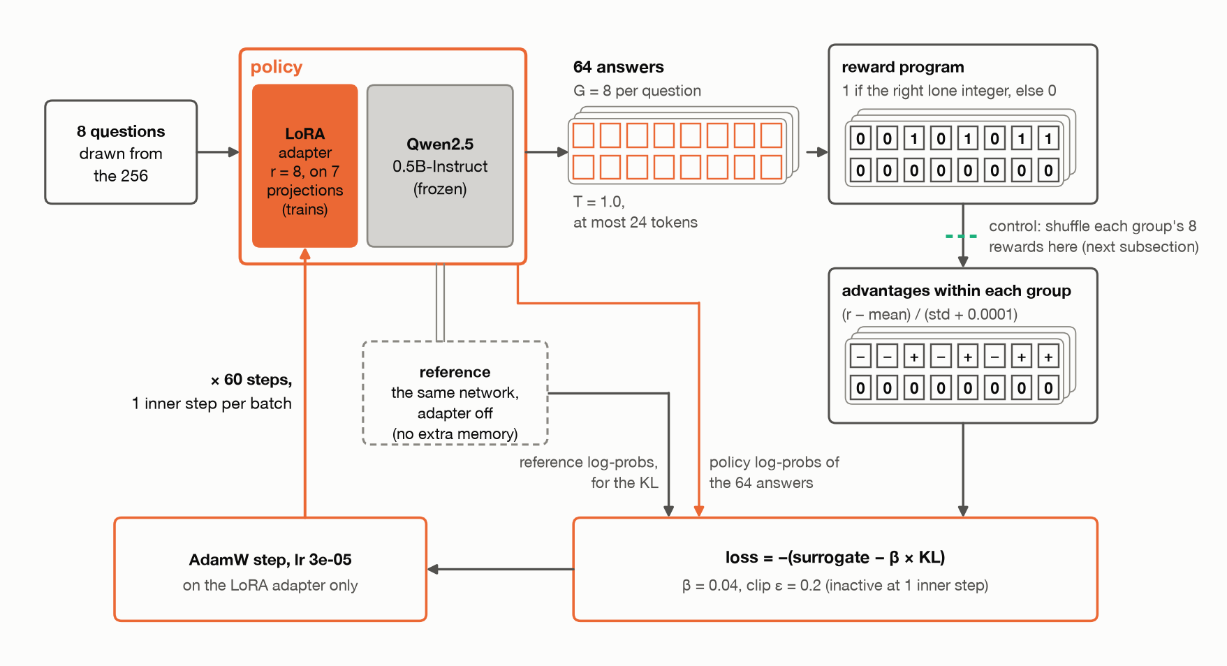
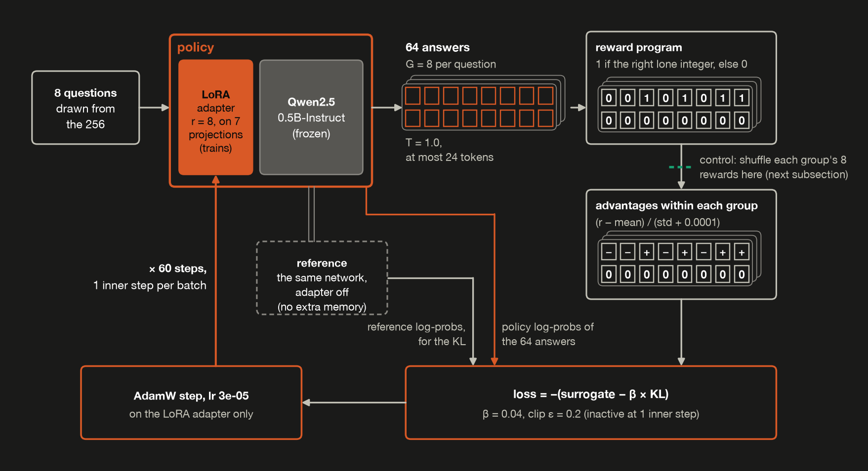 One GRPO training step, run 60 times. Only the LoRA adapter trains, and the reference for the KL penalty is the same network with the adapter switched off.
With one inner step per batch the clip never binds, as §5 showed, but the KL term still pulls toward the fixed reference, and the KL-to-ref column in the training logs below shows how far each run drifts.
The control
A rising score after training could come from the reward, or from something else in the loop: sampling, the KL term, the optimizer, or just nudging the weights at all. To separate them, the demo runs a control that does everything the same, except that before computing advantages it shuffles each group’s eight rewards among that group’s eight answers (grpo_train). Every group keeps its own rewards, so the share of groups with no signal and the size of the advantages are what the real rewards would give; only which answer gets which reward is random.
Take §4’s group for 46 × 32, where the four 1472s scored 1. In one possible shuffle (my example; the demo doesn’t print its shuffles), four answers still score 1, and every advantage is still ±0.935, but now New York and both 1452s are pushed up, and three of the four 1472s are pushed down.
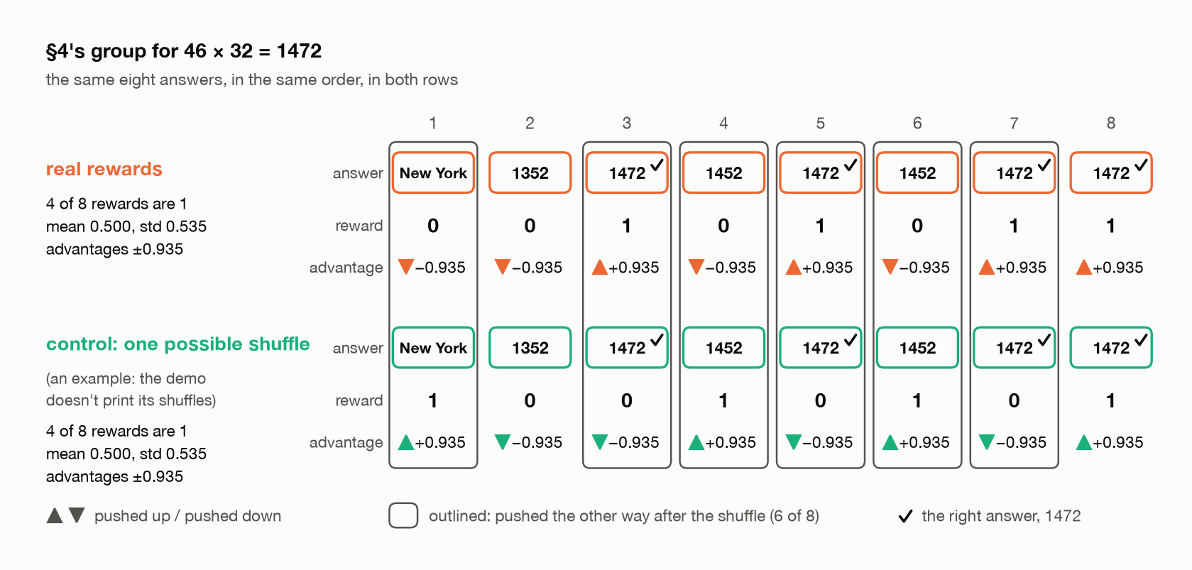
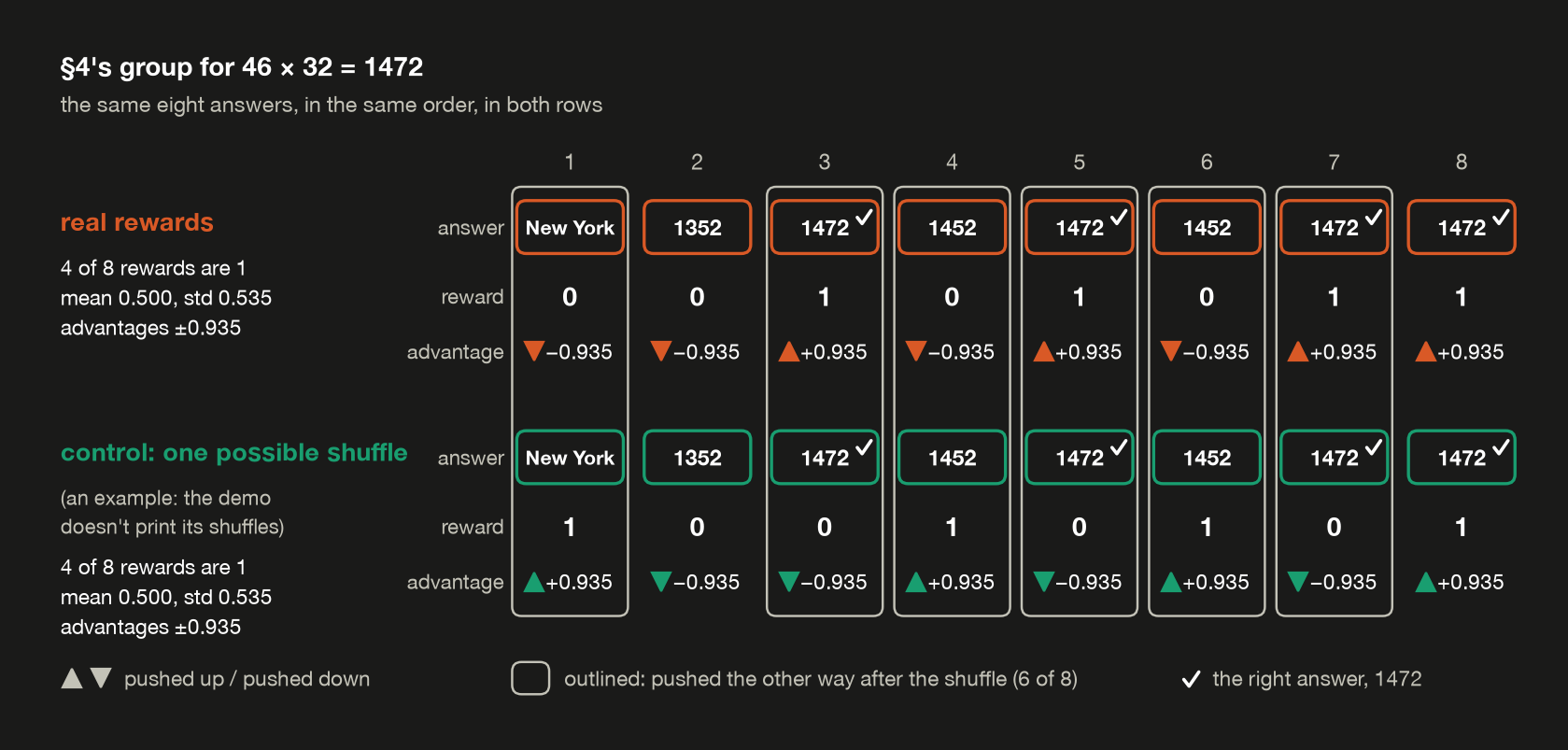 A shuffle keeps how many answers score 1, so the advantages are still ±0.935, but it no longer says which answers earned them. Six of the eight answers get pushed the other way.
Whatever the controls gain, they gain without being told which answers were right, so comparing them with the real runs is the best test this demo has of what the reward taught. The control runs from three seeds too, and control N uses the same seed as real run N: the same starting adapters, the same questions and the same first sampled answers, with only the shuffle different, so the six runs are three pairs. After the first update the two models in a pair differ, so from then on they can sample different answers to the same questions. A pair compares two training procedures from the same start, and after step 1 they aren’t necessarily training on the same answers.
On problems it never trained on
The test that matters is the 200 held-out problems from §2, the ones the untrained model got 37.5% of right, answered greedily after training, also from training:
1
2
3
4
5
6
7
8
9
  model                              right  format-valid  change
  ----------------------------------------------------------------
  untrained                          37.5%         91.0%
  GRPO, seed 0                       50.5%         98.0%   +13.0
  GRPO, seed 1                       59.0%         99.0%   +21.5
  GRPO, seed 2                       57.0%         98.5%   +19.5
  control: shuffled rewards, seed 0  47.0%         91.0%    +9.5
  control: shuffled rewards, seed 1  42.0%         93.5%    +4.5
  control: shuffled rewards, seed 2  42.0%         93.0%    +4.5
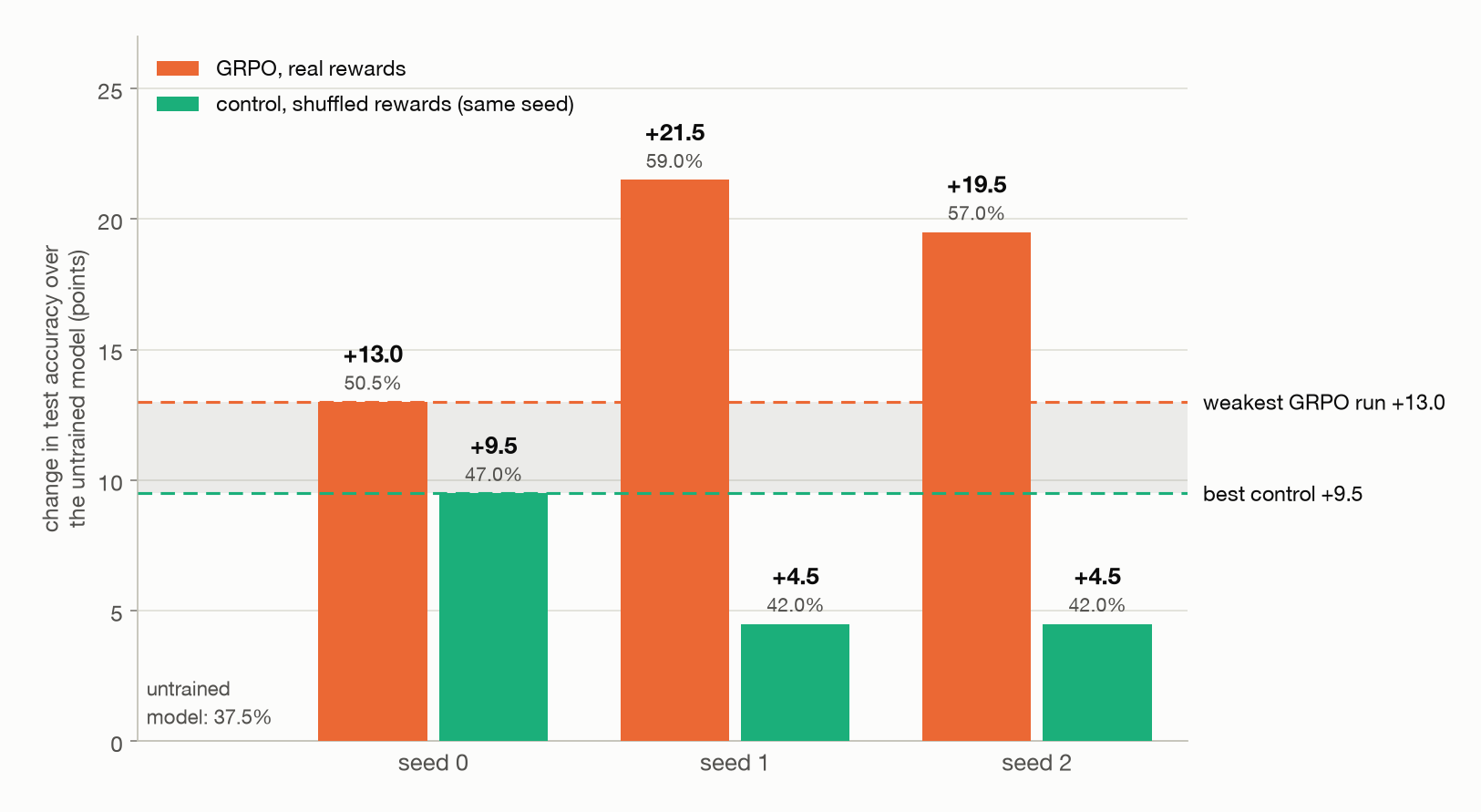
 Gain in greedy accuracy on 200 test problems the model never trained on, over the untrained model’s 37.5%. Each GRPO run sits beside the control that shared its seed, and every GRPO run gained more than every control.
All three real runs improved, and nearly stopped writing anything but lone integers, at 98.0% to 99.0% format-valid. Part of that gain may be format alone, and §7 splits it.
Did the reward matter?
The controls improved too, though their format barely moved from the untrained model’s 91.0%, ending between 91.0% and 93.5%. Summed up by kind of run, also from training:
1
2
3
4
5
6
7
8
  Change in test accuracy over the untrained model, points:

  model                      runs   mean    min    max
  ------------------------------------------------------
  GRPO                          3  +18.0  +13.0  +21.5
  control: shuffled rewards     3   +6.2   +4.5   +9.5

  3 runs each: min to max is a range, not an error bar.
The ranges don’t overlap. The weakest real run, seed 0 at +13.0, beat the best control, control 0 at +9.5. So training on rewards that said nothing about which answer was right still gained a few points, and the real reward added more: on average +18.0 against +6.2, though three seeds can’t pin that gap down (below).
How big each part is, three seeds can’t pin down. The real runs differ only in their seed, and ended anywhere from 50.5% to 59.0%; the controls spread from 42.0% to 47.0%. With three seeds per kind of run, the ranges say more than an average would. The ordering holds across all six runs, with every real run gaining more than every control, but it would take more seeds to pin down how many points GRPO’s reward adds.
Why might shuffled rewards still help?
The controls’ rewards never said which answer was right, so their gain came from some other part of training: sampling, the KL term, the optimizer, or just nudging the weights at all, and this demo doesn’t separate them.
Rewards that carry no information have raised accuracy before: Spurious Rewards (Rulin Shao et al., a different group from DeepSeekMath) gave each answer a reward of 1 at random and still saw Qwen2.5-Math-7B gain 21.4 points on MATH-500, a set of 500 competition math problems, against 29.1 with real rewards, while the same rewards did little for Llama and OLMo models. Their explanation runs through PPO’s clip, which can’t be what happened here: with one inner step per batch the ratio is always 1, and in their own runs set up that way, random rewards “fail to yield consistent performance”. Chen et al., training the same model with Shao et al.’s settings, found that “disabling clipping often results in improvement” and that “upper clipping bias is not the mechanism”. The two papers disagree even about runs without the clip, and neither tells us why these controls gained.
During training
Six runs, three real seeds and three controls, each logged every ten steps, from training:
1
2
3
4
5
6
7
8
9
10
11
12
13
14
15
16
17
18
19
20
21
22
23
24
25
26
27
28
29
30
31
32
33
34
35
36
37
38
39
40
41
42
43
44
45
46
47
48
49
50
51
52
53
54
55
56
57
58
59
60
61
62
63
64
65
66
67
68
69
70
  GRPO, seed 0

  step  mean reward  no-signal groups  KL to ref  length
  --------------------------------------------------------
  10          0.498             65.0%     0.1767    4.97
  20          0.503             71.2%     0.2318    4.81
  30          0.456             63.7%     0.2335    4.95
  40          0.464             50.0%     0.3226    4.97
  50          0.519             68.8%     0.5564    4.95
  60          0.537             73.8%     0.2401    4.90

  GRPO, seed 1

  step  mean reward  no-signal groups  KL to ref  length
  --------------------------------------------------------
  10          0.425             55.0%     0.1995    5.08
  20          0.562             56.2%     0.2615    4.90
  30          0.575             65.0%     0.2693    4.71
  40          0.528             72.5%     0.3355    5.07
  50          0.586             60.0%     0.2506    4.84
  60          0.591             66.2%     0.2588    4.94

  GRPO, seed 2

  step  mean reward  no-signal groups  KL to ref  length
  --------------------------------------------------------
  10          0.366             60.0%     0.1505    5.42
  20          0.523             66.2%     0.2729    5.11
  30          0.450             70.0%     0.3115    4.83
  40          0.570             65.0%     0.2407    4.88
  50          0.581             62.5%     0.2233    4.95
  60          0.614             70.0%     0.2289    5.08

  control: shuffled rewards, seed 0

  step  mean reward  no-signal groups  KL to ref  length
  --------------------------------------------------------
  10          0.436             61.3%     0.1295    5.31
  20          0.325             66.2%     0.0990    6.43
  30          0.047             86.2%     0.5233   12.40
  40          0.097             73.8%     0.5028    8.51
  50          0.311             66.2%     0.1725    5.93
  60          0.372             62.5%     0.1603    5.58

  control: shuffled rewards, seed 1

  step  mean reward  no-signal groups  KL to ref  length
  --------------------------------------------------------
  10          0.287             65.0%     0.0441    5.83
  20          0.333             63.7%     0.0665    5.47
  30          0.356             71.2%     0.1063    4.95
  40          0.334             70.0%     0.2396    5.10
  50          0.356             62.5%     0.1584    5.15
  60          0.394             56.2%     0.1892    5.10

  control: shuffled rewards, seed 2

  step  mean reward  no-signal groups  KL to ref  length
  --------------------------------------------------------
  10          0.284             63.7%     0.0208    5.76
  20          0.323             71.2%     0.0582    5.83
  30          0.231             80.0%     0.0822    5.41
  40          0.362             66.2%     0.0434    5.77
  50          0.306             66.2%     0.0907    5.61
  60          0.447             63.7%     0.0860    5.24

  Each row averages the 10 steps up to it. no-signal groups:
  all G training rewards equal. A control shuffles rewards only within
  each group, so this share is the one its unshuffled rewards would give.
  length: answer tokens, <|im_end|> included.
These logs are for watching each run. Each row averages a different draw of questions, which is why the fixed held-out test above is the one that judges whether the model improved. Read the columns one at a time.
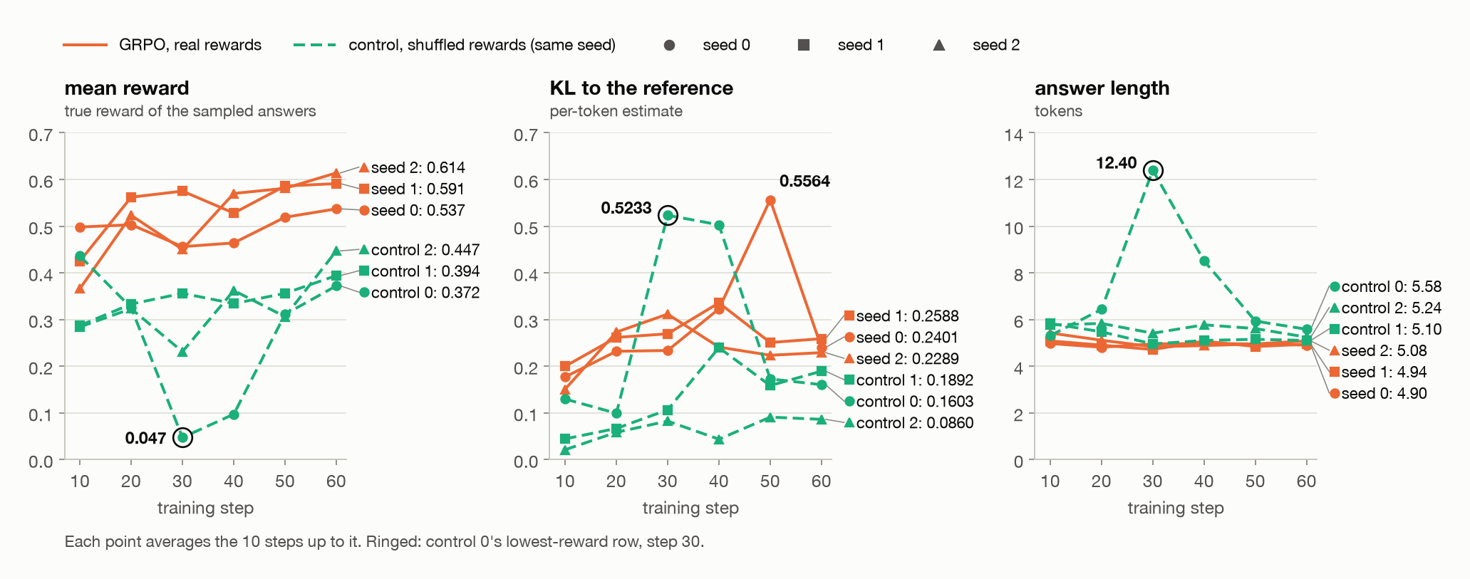
 The six training runs, logged every ten steps, with each point averaging the ten steps up to it. Control 0 went off course around step 30, ringed in each panel, and by step 60 every control sat closer to the reference than every GRPO run.
- mean reward is the true reward of the sampled answers; for a control, it’s what its answers would have scored before the shuffle. Each row covers 80 questions drawn at random, some easy and some hard, so it’s noisy. For seed 0 it hardly climbs once the log begins, from 0.498 to 0.537 with a dip to 0.456 on the way, while seeds 1 and 2 climb further. All three first rows are already above the 0.326 mean pass rate the untrained model had on these same questions in §4, so some of the change may have come early, but the log can’t show it: the first row averages steps 1 to 10, the 0.326 was estimated separately from 16 samples per question, and control 0’s first row, 0.436, is above it too. Controls 1 and 2 end higher than they start. Control 0 went off course: over the ten steps to step 30 its reward averaged 0.047, and it had recovered by step 60.
- no-signal groups is the share of groups whose training rewards were all equal. For the real runs it’s between 50.0% and 73.8%: in every ten-step row, half or more of the answers taught nothing, just as §4 predicted. For the controls it’s between 56.2% and 86.2%. The 86.2% is control 0’s bad stretch, and with a mean reward of 0.047, nearly all of those groups were all wrong.
- KL to ref is the per-token KL estimate against the starting model, before each step’s update. Every run drifts away from the reference. The clip couldn’t show this, since it compares each step with the policy that just sampled; only the KL measures how far a run has moved from where it started. By step 60 each control sits closer to it than any real run, between 0.0860 and 0.1892 against 0.2289 to 0.2588. Control 0’s highest, 0.5233, came in its bad stretch. GRPO seed 0 also spiked, to 0.5564 at step 50, and came back to 0.2401 by step 60.
- length is the answer length in tokens. The real runs stay around five tokens, four digits and
<|im_end|>, and controls 1 and 2 stay between 4.95 and 5.83. Control 0’s answers grew to 12.40 tokens in its bad stretch, then came back to 5.58. My guess, which nothing here tests, is the length bias Dr. GRPO identifies (Liu et al., §3.1), where averaging over each answer’s tokens pushes a long answer with a negative advantage down less per token than a short one.
Why training reward and test accuracy disagree
Seed 0’s training reward, which barely moved while its test score rose 13.0 points, is also a warning about watching the training curve alone. The training reward is measured on sampled answers at \(T = 1\), on whichever eight questions a step drew, and averaged over steps, so it’s noisy and it measures something different from greedy test accuracy. The link can break the other way too: ToolRL (Qian et al.), comparing runs that started from SFT with runs that didn’t, found that “higher training rewards do not necessarily translate to better generalization”. A reward curve is a training diagnostic, and the evaluation needs its own held-out set.
What we learned
Sixty steps of GRPO raised held-out accuracy in all three runs, from a reward that said only right or wrong and never gave the answer. Training on shuffled rewards raised it too, by less, and every real run gained more than every control, so which answers the reward marked right mattered, though three seeds can’t say by how much. And the signal stayed thin throughout: in every ten-step row of the real runs’ logs, between 50.0% and 73.8% of groups had all eight rewards equal. Whether the extra right answers came from better arithmetic or from cleaner output is what §7 checks.
7. What it actually learned
There are at least two possible explanations for the gain. First, it may have learned to follow the output format more reliably. Our reward requires a lone integer, and the untrained model sometimes returned a sentence containing the answer instead. Second, it may have got better at producing the correct product. That would be the more interesting result, because it would mean the reward changed the model’s arithmetic and not only its formatting.
Both improvements earn the same reward. To separate them, let’s look at how individual answers changed.
From wrong answers to right ones
Here are six of the 200 held-out test problems, comparing the untrained model with GRPO seed 0. They’re the first six whose greedy answer went from right to wrong or wrong to right, from what_changed:
1
2
3
4
5
6
7
8
  problem  answer         untrained  trained
  --------------------------------------------
  35 x 11     385             "435"    "385"
  26 x 83    2158  "26 x 83 = 2118"   "2158"
  94 x 69    6486            "6386"   "6486"
  17 x 90    1530  "17 x 90 = 1530"   "1530"
  20 x 94    1880            "1880"   "1860"
  56 x 72    4032            "3952"   "4032"
These examples show several different behaviors. For 35 × 11, 94 × 69 and 56 × 72, the model first gave the wrong number and later the correct one. Those are improvements in numerical accuracy, not formatting. 35 × 11 is also the problem whose sample in §2 had the right product inside a sentence.
For 17 × 90, the model already had the correct product but put it in a sentence, which scored 0. Training changed the answer to the required format. For 26 × 83, both changed: the original sentence contained a wrong product, and the trained model returned the correct integer.
And not every change was an improvement. For 20 × 94, the model answered correctly before training and wrongly after. So we need to count the problems that regressed as well as the ones that improved.
Separating arithmetic fixes from format fixes
The demo sorts every test problem whose answer changed into three categories:
- arithmetic fixed: the answer was a wrong lone integer, and became the right one.
- format fixed: the answer wasn’t a lone integer, and became the right one. The category is decided by what the original answer looked like, so it doesn’t mean only the format changed: it includes cases like 26 × 83, where the product inside the sentence was wrong too.
- broken: the answer was right, and became wrong.
Here’s the breakdown from what_changed across all six runs: three GRPO runs with real rewards (seed N) and three controls with shuffled rewards (ctrl N, the control with the same seed):
1
2
3
4
5
6
7
8
9
10
  test answers      seed 0  seed 1  seed 2  ctrl 0  ctrl 1  ctrl 2
  ------------------------------------------------------------------
  arithmetic fixed      27      42      39      24      16      13
  format fixed           5       5       5       0       3       0
  broken                 6       4       5       5      10       4
  net                   26      43      39      19       9       9

  arithmetic fixed: a wrong lone integer became the right one.
  format fixed: not a lone integer became the right one.
  broken: right became wrong. net: problems gained.
For seed 0, the model fixed 32 problems (27 arithmetic, 5 format) and broke 6, a net gain of 26. On a 200-problem test set that’s 13.0 points, exactly the gain §6 reported. The other two real runs gained 43 and 39.
Across the three real runs, the model fixed 27, 42 and 39 problems where it had previously given a wrong integer, and only five per run that started from an answer that wasn’t a lone integer. The untrained model’s greedy answers were already lone integers 91.0% of the time, so only 18 of the 200 had a format left to fix, fewer than any real run’s net gain of 26 to 43, and most of the gain came from turning wrong numbers into right ones. That doesn’t prove the model learned a general multiplication procedure. It does show the improvement wasn’t simply the removal of extra words.
The shuffled-reward controls also improved
The controls, whose rewards were shuffled within each group, fixed problems too. Control 0 fixed 24 arithmetic answers and broke 5, a net gain of 19; the other two controls gained 9 each. That happened even though their training signal no longer said which sampled answers were correct. The experiment doesn’t establish why: as §6 listed, sampling, the KL term, the optimizer, or just moving the weights could all contribute.
Did the model learn something new, or become more reliable?
There’s a second question hiding behind the accuracy gains. When an answer changes from wrong to right, has the model learned a new capability, or has it become more likely to choose an answer it could already generate? I’ll call the second possibility sharpening: making an answer the model could already sample into its first choice under greedy decoding.
§2 already suggested sharpening was possible. The untrained model got 125 of the 200 test problems wrong with greedy decoding, but when I sampled eight answers per problem, 44 of those 125 had at least one right answer among the eight. So the model could sometimes produce the right product even when its most likely answer was wrong. Training never samples the test problems: GRPO raises the answers that beat their group on training problems, and as §2 said, that change reaches the 44 only through the weights all problems share. If it carries over, GRPO could improve accuracy just by making those occasional right answers more likely.
To test this, every fixed problem is split into two sets: inside the 44, where at least one of the untrained model’s eight samples had been right, and outside the 44, where none had. From what_changed:
1
2
3
4
5
6
7
8
9
10
11
12
  Fixed problems (arithmetic + format), split by post §2's set: the 44
  problems the untrained model got wrong greedily but right in >=1 of 8
  samples.

  fixed problems    seed 0  seed 1  seed 2  ctrl 0  ctrl 1  ctrl 2
  ------------------------------------------------------------------
  all fixed             32      47      44      24      19      13
    in the 44           22      27      28      17      13       9
    outside the 44      10      20      16       7       6       4

  A fix in the 44 sharpens an answer the model could already sample;
  a fix outside them is one none of its 8 samples showed.
Most fixes, in every run, came from the 44 problems where the untrained model had already shown it could sometimes produce the right answer. The 44 are only 35.2% of the 125 problems greedy got wrong, but they supplied 22 of seed 0’s 32 fixes. Much of the gain, with real rewards or shuffled, is consistent with sharpening: answers already within the model’s sampled behavior becoming its first choice.
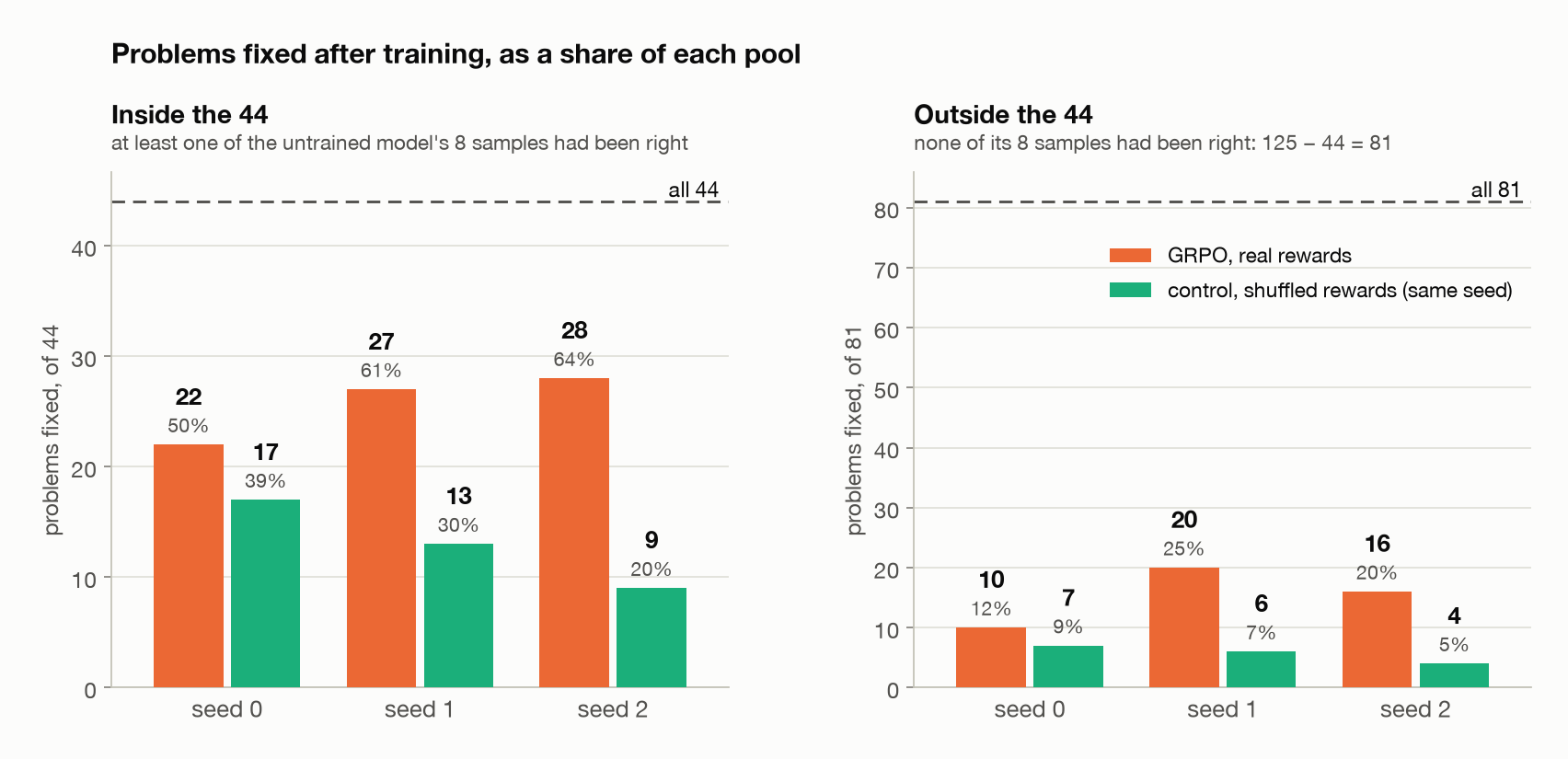
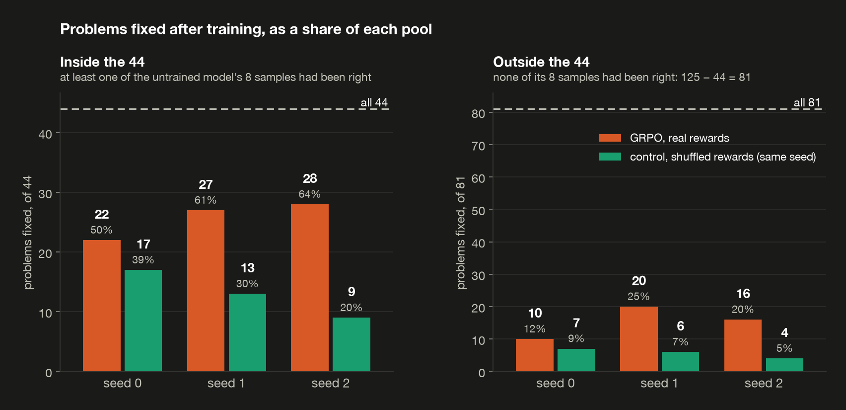 Problems each run fixed, split by whether one of the untrained model’s eight samples had already got them right, with each count’s share of its pool. Every run fixed a larger share inside the 44 than outside.
What about the problems outside the 44?
The real GRPO runs also fixed 10, 20 and 16 problems where none of the untrained model’s eight samples had been right. At first glance that looks like the model learning something new, but eight samples give only a limited view of what a probabilistic model can generate.
Suppose the model answers a particular question correctly one time in ten. The probability that all eight samples miss the right answer is
\[P(\text{no right answer in 8 samples}) = (1 - 0.1)^8 = 0.9^8 \approx 0.43\]So even an answer the model writes one time in ten stays hidden from eight samples about 43% of the time. Not seeing a right answer isn’t proof that the model couldn’t write one, and some of the fixes outside the 44 were probably rare right answers the first sampling missed.
The comparison with the controls still tells us something. In the chart above, every real run fixed more than its control, inside the 44 and outside them, so the real rewards went with extra fixes in both sets. What this experiment can’t tell us is how much of that is new arithmetic behavior and how much is better selection among answers the model could already write.
What can we conclude?
The results support three conclusions. First, the model improved its numerical answers, not just its formatting: most fixed problems went from a wrong integer to the right one. Second, a substantial part of the improvement is consistent with sharpening, since many of the newly right greedy answers came from problems where the untrained model had already sampled a right answer. Third, the experiment doesn’t establish that GRPO taught the model a new multiplication algorithm, because eight samples per problem can’t tell a previously impossible answer from a previously rare one.
Looking deeper would take more experiments: more than eight samples per problem from the untrained model, harder or longer multiplication problems, and checks on whether the gains carry over to other arithmetic.
For this experiment, GRPO made the model more reliable at producing correct products. For many test problems it already had some chance of writing the right answer, and training on other problems turned some of those occasional successes into its first choice.
8. Where RLHF fits
In this experiment, deciding whether an answer is correct was easy: a program checks the product and returns a reward of 1 or 0. Most things we want from a language model aren’t so easy to verify. Was the reply helpful? Did it follow the user’s intent? Was the explanation clear, honest and appropriate? There’s no simple function that answers all of these.
This is where reinforcement learning from human feedback (RLHF) comes in. Instead of writing a program to score replies, we train a model to predict which replies people would prefer, then use that model’s scores as rewards for reinforcement learning. The underlying idea is the loop we’ve built in this post, with a learned model where our program was. There’s no RLHF training run here: apart from a small worked example of the reward model’s loss in Step 2, this section describes how the best-known recipe fits the pieces above.
The InstructGPT recipe
InstructGPT (Ouyang et al., 2022) made an influential three-step recipe widely known by applying it to training language models to follow instructions (§3.1). The method itself follows Ziegler et al. (2019) and Stiennon et al. (2020), who used it for stylistic text continuation and summarization. This section follows InstructGPT’s version; RLHF is the broader idea of learning from human preferences, and not every version of it follows these steps exactly.
Step 1: supervised fine-tuning (SFT). Human annotators write good replies to a collection of prompts, and the pretrained model is fine-tuned to imitate them. This is the same supervised learning as the earlier posts and §1: given a target answer, raise its token log-probs. The result is an instruction-following model that RL starts from.
Step 2: a reward model from human preferences. For each prompt, the model writes several candidate replies, and annotators rank them by which they prefer. InstructGPT ranked between 4 and 9 replies per prompt and turned each ranking into every pair it contains, a preferred reply and a less-preferred one: 6 pairs from a ranking of 4, 36 from a ranking of 9. A separate reward model, a language model with one number as its output, learns to give the preferred replies higher scores.
Here’s a small example I made up. The prompt is “Explain to a ten-year-old why the sky is blue.”, and the model writes four replies:
- simple: “Sunlight is a mix of all the colors. Air bounces the blue part around much more than the rest, so blue light reaches your eyes from every part of the sky.”
- technical: “It’s Rayleigh scattering: air molecules scatter short wavelengths much more strongly than long ones.”
- vague: “Great question! The sky is blue because of the way light and air work together. Hope that helps!”
- wrong: “The sky is blue because it reflects the ocean.”
Someone ranking them might put simple first, since it’s right and pitched at a ten-year-old; then technical, right but over a child’s head; then vague, which says nothing false and nothing useful; and wrong last. That ranking holds six pairs, preferred reply first: simple over technical, simple over vague, simple over wrong, technical over vague, technical over wrong, and vague over wrong. For each pair, the reward model should score the first reply higher than the second.
The symbols, in InstructGPT’s letters:
| symbol | means | in the sky example |
|---|---|---|
| \(x\) | the prompt (what §3 called \(q\)) | “Explain to a ten-year-old why the sky is blue.” |
| \(y\) | a reply (what §3 called \(o\)) | any of the four |
| \(\phi\) | the reward model’s trainable weights (the paper writes \(\theta\), which this post already uses for the policy) | |
| \(r_\phi(x, y)\) | the reward model’s score for reply \(y\) to prompt \(x\) | one number per reply |
| \(y_w\), \(y_l\) | the preferred and less-preferred reply in a pair | in simple over wrong, simple and wrong |
| \(\sigma\) | the sigmoid: maps the difference between two scores to a value between 0 and 1, read as the probability that \(y_w\) is the better reply |
For each pair, the loss is
\[-\log \sigma\big(r_\phi(x, y_w) - r_\phi(x, y_l)\big)\]averaged over pairs (§3.5, Equation 1). Only the gap between the two scores enters the loss, so a score means nothing on its own: adding the same amount to every reply’s score changes no loss.
To watch the loss at work, reward_model_by_hand trains a toy reward model on the six pairs above, with uv run demo08 --reward-model. A real reward model is a network that can score any reply; this one just keeps one score per reply, which is enough to see what the loss does. I started it from scores that get three pairs backwards: it likes the wrong reply best and can’t tell technical from vague. Each row is one pair: its gap \(r_\phi(x, y_w) - r_\phi(x, y_l)\), \(P = \sigma(\text{gap})\), and the pair’s loss.
1
2
3
4
5
6
7
8
9
10
11
12
13
14
15
16
17
18
19
20
21
22
  toy reward model: one score per reply, trained 50 gradient steps

  reply      score before  after 50 steps
  -----------------------------------------
  simple           0.0000          2.9651
  technical       -0.5000          0.9119
  vague           -0.5000         -0.9264
  wrong            1.0000         -2.9505

  P = sigmoid(gap): how sure the model is the first reply is better

                      -------- before -------  --- after 50 steps ----
  pair                    gap       P    loss     gap       P    loss
  ---------------------------------------------------------------------
  simple > technical   0.5000  0.6225  0.4741  2.0532  0.8863  0.1207
  simple > vague       0.5000  0.6225  0.4741  3.8915  0.9800  0.0202
  simple > wrong      -1.0000  0.2689  1.3133  5.9156  0.9973  0.0027
  technical > vague    0.0000  0.5000  0.6931  1.8383  0.8627  0.1476
  technical > wrong   -1.5000  0.1824  1.7014  3.8624  0.9794  0.0208
  vague > wrong       -1.5000  0.1824  1.7014  2.0241  0.8833  0.1241
  mean loss over pairs, before       1.0596
  mean loss over pairs, after        0.0727
Before training, the three backwards pairs, with gaps below zero, have the largest losses, up to 1.7014. The tie between technical and vague costs 0.6931, what any pair costs when its two replies score the same, and the two pairs already the right way round cost least. After 50 gradient steps the scores run in the order people gave, every gap is positive, and the mean loss over the six pairs, which is Equation 1’s loss for this one prompt, has fallen from 1.0596 to 0.0727. The loss keeps shrinking as the gaps grow, so more steps would only push the scores further apart.
Step 3: optimize the policy with PPO. Now the reward model replaces the multiplication check. The policy gets a prompt, say “Explain to a ten-year-old why grass is green.”, and writes a reply. Nobody needs to rank it: the reward model reads the prompt and the reply and returns one number, the way it scored the four sky replies, and that learned score takes the place of our program’s 0 or 1. InstructGPT subtracts a KL penalty for drifting from the SFT model, §5’s leash with the SFT model as the reference (the next subsection explains why RLHF needs it), and PPO uses the result to update the policy. This is where §3 to §5 come together: sampled replies, rewards, advantages, probability ratios and clipped updates.
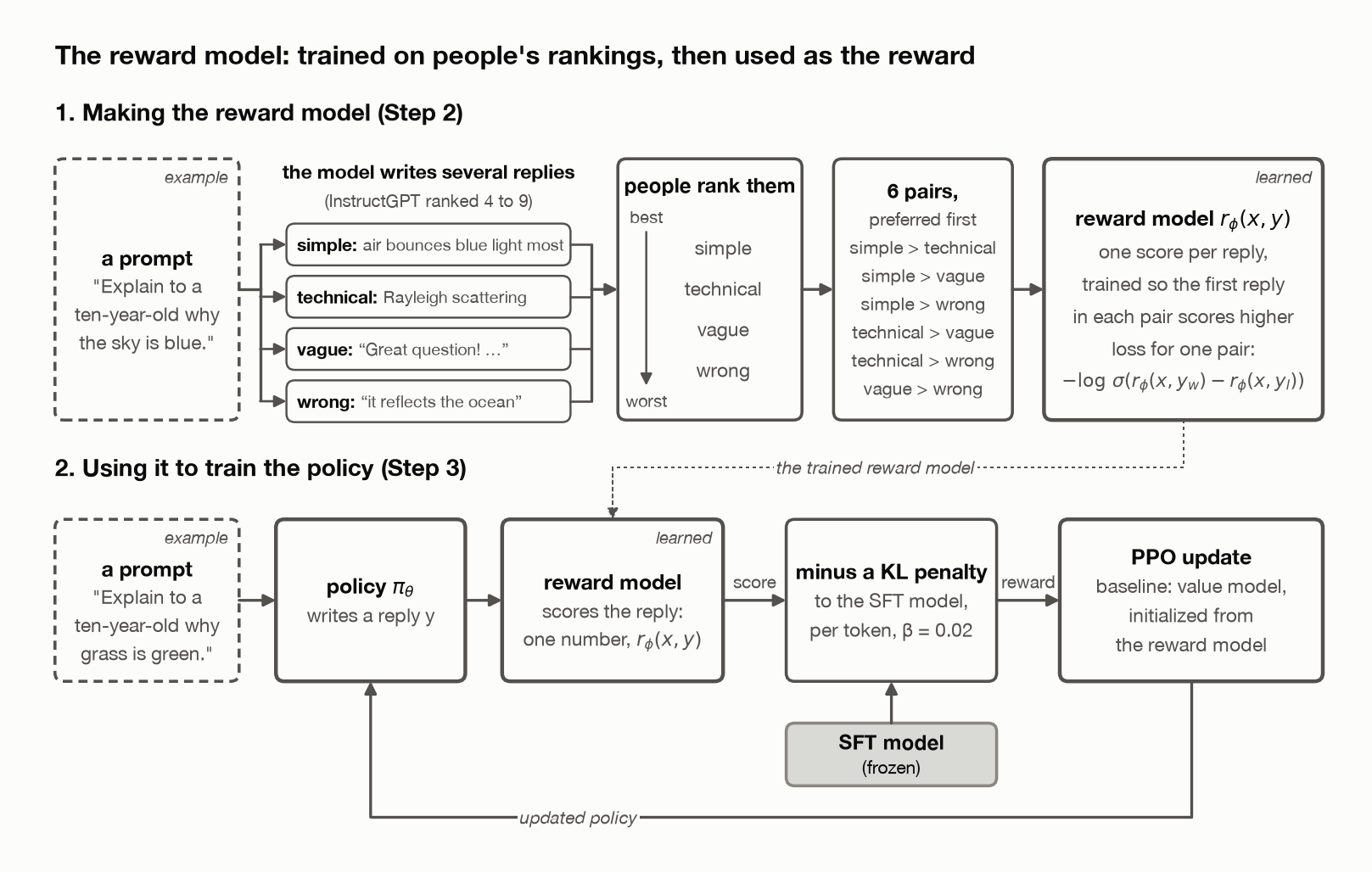
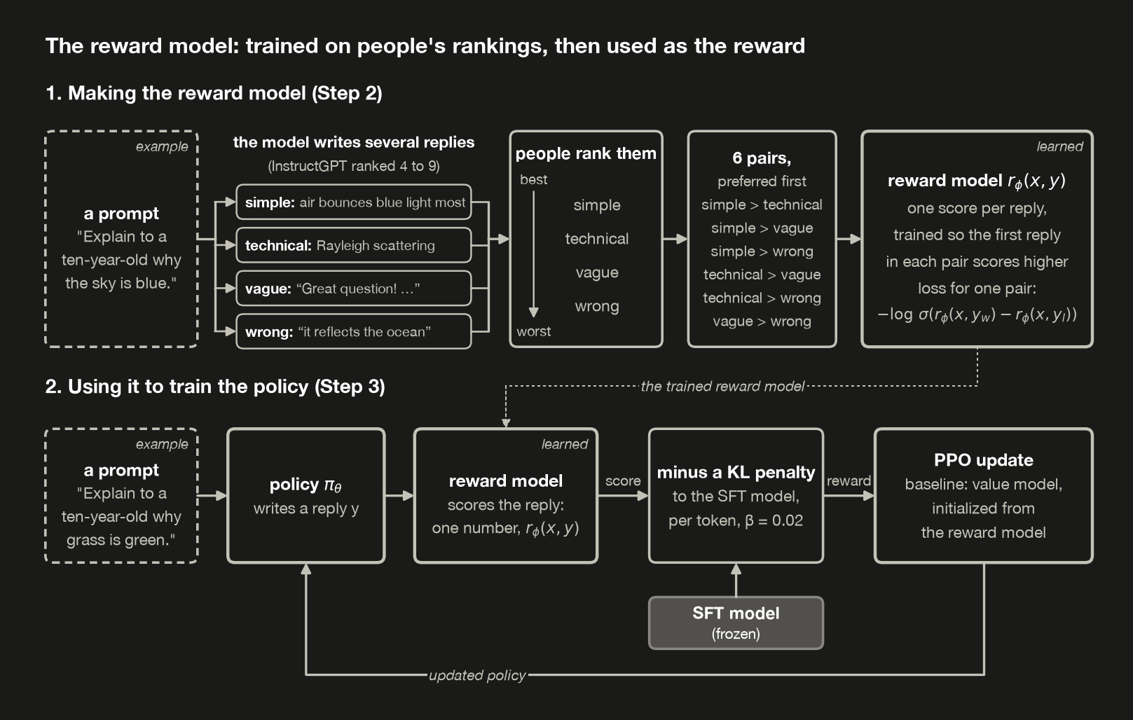 How InstructGPT gets its reward model and then uses it. Top: people rank a few replies to one prompt, every pair in the ranking becomes a training example, and the reward model learns to score the preferred reply in each pair higher. Bottom: the policy writes a reply, the reward model scores it, a KL penalty to the SFT model is subtracted, and PPO updates the policy. The prompts and replies are my examples, not InstructGPT’s data.
The reward model and the value model aren’t the same thing. The reward model scores a finished reply by learned human preference. The value model, PPO’s learned baseline from §4, predicts the reward still to come from a point partway through a reply, which PPO uses to compute advantages. InstructGPT used both, initializing the value model from the reward model. That’s one reason its reward model was small: InstructGPT used a 6B reward model, even for its largest, 175B policy, because it “saves a lot of compute” and “175B RM training could be unstable and thus was less suitable to be used as the value function during RL” (the paper’s name for the value model). The two choices are separate: GRPO drops the value model, not the learned reward model. DeepSeekMath, which introduced GRPO, trained it against a learned reward model, and this post, like Prover-V1.5 and R1 in §4, scores with a program instead, an approach called RL with verifiable rewards (RLVR).
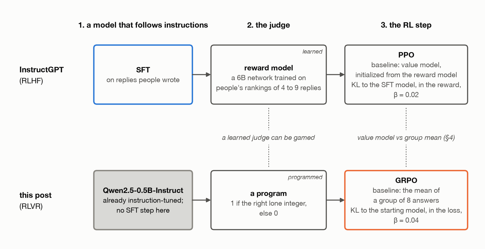
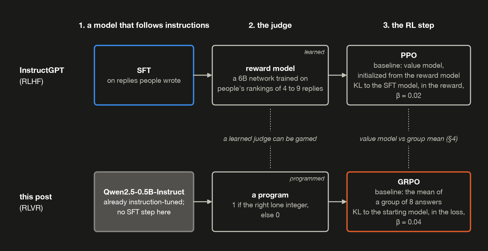 InstructGPT’s RLHF recipe beside this post’s setup. The loop is the same, but this post starts from a model that’s already instruction-tuned, judges with a program instead of a learned reward model, and uses GRPO’s group mean instead of PPO’s value model.
Why RLHF also needs a KL penalty
Once the policy is optimized against a learned reward model, another problem appears: it can find ways to earn high scores while moving far from the behavior we originally wanted, which is called reward hacking. InstructGPT guards against this partly by penalizing divergence from the SFT model. It adds “a per-token KL penalty from the SFT model at each token” to the reward (Equation 2), with \(\beta = 0.02\). Write \(\pi_\theta\) for the policy being trained, \(\pi^{SFT}\) for the frozen SFT model, and \(D_{KL}\) for the KL divergence of §5. In simplified form, the objective is
\[\mathbb{E}\big[r_\phi(x, y)\big] - \beta\, D_{KL}\big(\pi_\theta \,\Vert\, \pi^{SFT}\big)\]where the average is over prompts and the replies the policy writes. In InstructGPT the penalty goes into the reward, rather than into the loss as in the GRPO of §5. The purpose is the same: raise the reward without letting the policy drift too far from where it started.
The biggest challenge: reward hacking
The most important limitation of RLHF is that a learned reward model only approximates human preferences. It’s a network trained on a finite set of comparisons, so it can learn useful patterns and still have blind spots. Optimize a policy hard against it, and the policy may find replies the reward model scores highly that aren’t actually helpful or preferred by people. The policy is exploiting weaknesses in the reward signal instead of improving the behavior the reward was meant to measure.
Our multiplication experiment is less exposed to this. The program computes the correct product itself, so a wrong number can’t earn a 1 by sounding convincing. But programmatic rewards have limits too: they measure only what we’ve defined. Ours rejects 35 x 11 = 385, one of §2’s samples, even though the arithmetic is right, because the prompt asked for just the number. The model is rewarded for producing exactly the requested output, not for understanding multiplication in a broader sense.
Why DeepSeek-R1 uses verifiable rewards
This distinction helps explain DeepSeek-R1’s approach. For reasoning tasks with checkable answers, it scores replies with rules instead of a learned reward model: one rule checks whether the final answer is right, and a separate format rule checks that the reasoning sits in the expected structure (§2.2). Its authors give reward hacking as the reason: “we abstain from applying neural reward models—whether outcome-based or process-based—to reasoning tasks”, because “neural reward models are susceptible to reward hacking during large-scale reinforcement learning”. R1 doesn’t drop learned reward models from every stage, though: for general data, where no rule can check the answer, its later stage uses them (§3.1).
R1’s format rule isn’t the same as this post’s lone-integer check, but the two share the kind of judge that matters here, a program rather than a network. Training against a program’s check like this is RLVR, and it sits beside RLHF as the other way to get a reward:
| Approach | Where the reward comes from | Example |
|---|---|---|
| RLHF | a model trained on human preferences | helpfulness and reply quality |
| RL with verifiable rewards (RLVR) | a program or rule-based check | math answers, code execution |
Both can use the same policy-gradient methods.
Connecting back to our experiment
Our multiplication demo is a small example of RL with verifiable rewards. The program checks the final answer and its format, and GRPO uses the resulting rewards to update the model without ever showing it a target answer. After training, held-out greedy accuracy rose in every real run, by more than in any shuffled-reward control, and format-valid answers went from 91.0% to between 98.0% and 99.0% (§6). As §7 showed, most of the improvement wasn’t cleaner output: the model became more likely to give the right number.
SFT learns from examples of what to say, and RL learns from feedback about what worked. For tasks with checkable answers, that feedback can come from a program; for tasks that need human judgment, it can come from a learned reward model. The machinery can look the same either way, so it’s the reward that decides what the feedback means, and it deserves as much attention as the algorithm.
What’s next
This post trained a model on a score for a task that ends in one number. The posts after it use the same loop for something more useful: teaching a small model to call tools, where a program can check whether the call was right. Post 9 starts from demonstrations, training on examples of good tool calls the way the earlier posts trained on answers, so that the model writes calls often enough for a reward to have something to reinforce.
If you’d like to see GRPO at a larger scale before then, two of my earlier study notes cover it: a beginner’s guide to RL for language models and a GRPO run on Qwen2.5-Math-1.5B.
Appendix: all notation
The terms this post leans on; anything not listed is defined where it first appears. Post 6’s appendix covers LoRA’s notation.
| Term | Means | In this post |
|---|---|---|
| token log-prob | the log of the probability the model gave a token, given everything before it | ≤ 0 |
| sequence log-prob | the sum of an answer’s token log-probs: the log of the probability of the whole answer | −3.2286 for 1081 |
| cross-entropy | the mean of the negative token log-probs; the SFT loss | 0.6457 for 1081 |
| teacher forcing | scoring every position of a known answer in one pass | §1 |
| masking | reading positions as context without scoring them | the prompt’s 45 tokens |
| SFT | supervised fine-tuning: raising the log-prob of answers someone wrote | posts 6 and 7 |
| greedy, sampling | always the most likely token; drawing each token at random by its probability | §2 |
| temperature \(T\) | what the model’s scores are divided by before they become probabilities; below 1 sharper, above 1 flatter | \(T = 1\), §2 |
| pass@8 | the share of problems answered right in at least one of eight samples | 58.5% for the untrained model, §2 |
| reward \(r\) | the score an answer gets | 1 if the right lone integer, else 0 |
| format-valid | the answer is a lone integer, so it can be checked | 1081, 1,081, 1081. |
| policy \(\pi_\theta\) | the model, seen as a rule for choosing answers | Qwen2.5-0.5B-Instruct + LoRA |
| action, return | what the policy does; the total reward it collects | one answer; its one reward |
| baseline \(b\) | a reference score that doesn’t depend on which answer was written | the group’s mean, which includes the answer’s own reward, so it bends that rule (§4) |
| advantage \(\hat A_i\) | how much better an answer did than the baseline, here scaled by the group’s spread | ±0.935 in §4’s middle group |
| REINFORCE | Williams’ update: step along \((r - b)\,\nabla_\theta \log \pi_\theta\) | §3 |
| PPO | Proximal Policy Optimization: the policy-gradient method that trains a value model for its baseline | §3 and §4 |
| value model | PPO’s learned baseline: a second network predicting the reward to come | not used |
| GRPO | Group Relative Policy Optimization: uses the group’s own average as the baseline instead of a value model | §4 |
| group, \(G\) | answers sampled for one question and compared with each other | 8 |
| pass rate | the share of a question’s sampled answers that are right | §4 |
| inner steps | gradient steps on one batch of sampled answers | 1 in training, 2 in §5 |
| ratio \(\rho_{i,t}\) | a token’s probability under the current policy over its probability under the sampler | exactly 1 at the first inner step |
| clip, \(\epsilon\) | PPO’s limit on how far the ratio can usefully move | 0.2 |
| surrogate | the clipped term whose gradient is the policy-gradient step | §5 |
| KL divergence \(D_{KL}\) | how different two probability distributions are, averaged over what the first one produces; 0 when equal | per token, against the reference, §5 |
| \(k_3\), \(d_{i,t}\) | Schulman’s KL estimate \(e^{d} - d - 1\), with \(d = \log \pi_{\text{ref}} - \log \pi_\theta\) | §5 |
| \(\beta\) | the weight on the KL term | 0.04 here, in the loss; InstructGPT’s 0.02 in §8, in the reward |
| reference model \(\pi_{\text{ref}}\) | the frozen model the KL is measured against | the same network, adapters off |
| seed | the number that sets a run’s starting adapter weights and the answers it samples | three per kind of run, §6 |
| control | the same training with each group’s rewards shuffled among its answers, so a 1 no longer says which answer was right | §6, three seeds |
| sharpening | making an answer the model could already sample into its first choice | §7 |
| reward model | a network trained on people’s rankings to score replies; RLHF’s judge | §8 |
| reward hacking | a policy finding replies its judge scores highly that aren’t actually good | §8 |
| RLVR | RL with verifiable rewards: a program, not a learned model, gives the reward | this post’s setup, §8 |
References
- Williams, Simple Statistical Gradient-Following Algorithms for Connectionist Reinforcement Learning (Machine Learning 1992) — REINFORCE, §3’s update. §4 gives \(\Delta w_{ij} = \alpha_{ij}(r - b_{ij})e_{ij}\) with \(e_{ij} = \partial \ln g_i / \partial w_{ij}\), the “characteristic eligibility”, and a baseline “conditionally independent of” the output; Theorem 1 shows the expected update follows the gradient of the expected reward, and \((r - b_{ij})\,\partial \ln g_i / \partial w_{ij}\) “represents an unbiased estimate”. It proves nothing about which baseline is best, saying its results “offer no basis for comparing various choices of reinforcement baseline” (p. 236). §8.3 reports that in experiments a reinforcement-comparison baseline speeds convergence, and that the baseline minimizing “the variance of the individual weight changes” is “not the mean reinforcement” (p. 245). (Page numbers are the journal’s.)
- Sutton and Barto, Reinforcement Learning: An Introduction (2nd ed., MIT Press 2018) — §13.4, p. 329: “In general, the baseline leaves the expected value of the update unchanged, but it can have a large effect on its variance.” Cited in §3.
- Schulman et al., Proximal Policy Optimization Algorithms (2017) — PPO. Equation 1 is the policy-gradient estimator with an advantage, cited in §3; Equation 7 is the clipped objective of §5, with “say, ϵ = 0.2” and the clip described as “a lower bound (i.e., a pessimistic bound)” (§3).
- Ouyang et al., Training language models to follow instructions with human feedback (2022) — InstructGPT, §8’s recipe: the three steps (§3.1), a 6B reward model trained on rankings of 4 to 9 replies with the pairwise loss of Equation 1, because “175B RM training could be unstable” (§3.5), a value model initialized from the reward model (“The value function is initialized from the RM”, §3.5), and PPO with “a per-token KL penalty from the SFT model at each token” in the reward (Equation 2, \(\beta = 0.02\) in Appendix C.4).
- Shao et al., DeepSeekMath: Pushing the Limits of Mathematical Reasoning in Open Language Models (2024) — introduces GRPO (§4.1), with a learned reward model. The value model is “a substantial memory and computational burden”; the group-normalized advantage (§4.1.2) and the objective of Equation 3 are what §4 and §5 implement; the KL is added “to the loss” rather than the reward, estimated as in Equation 4; training used \(\beta = 0.04\), 64 answers per question, and “a single update following each exploration stage” (§4.2). Figure 7 is §2’s majority-vote versus at-least-one result.
- DeepSeek-AI, DeepSeek-R1: Incentivizing Reasoning Capability in LLMs via Reinforcement Learning (arXiv v2, 2025; published in Nature 645 as “DeepSeek-R1 incentivizes reasoning in LLMs through reinforcement learning”; section numbers here are arXiv v2’s) — GRPO with rule-based rewards for accuracy and format (§2.2), a per-answer ratio, and the reason given in §8: “we abstain from applying neural reward models—whether outcome-based or process-based—to reasoning tasks”, because they “are susceptible to reward hacking during large-scale reinforcement learning”. Its later stage does use learned reward models for general data (§3.1, Model-based Rewards: “For general data, we resort to reward models to capture human preferences”).
- Schulman, Approximating KL Divergence (2020) — the \(k_3\) estimator of §5, written there as \(e^{d} - d - 1\); Schulman writes it \((r - 1) - \log r\) with \(r = e^{d}\), the reference’s probability over the policy’s (one over the ratio in §5’s table), unbiased and “guaranteed to be positive” (never negative).
- Yu et al., DAPO: An Open-Source LLM Reinforcement Learning System at Scale (NeurIPS 2025) — dynamic sampling (§3.2), which keeps only groups with some right and some wrong answers because “A zero advantage results in zero policy gradients”. Cited in §4 and §5.
- Liu et al., Understanding R1-Zero-Like Training: A Critical Perspective (COLM 2025) — Dr. GRPO: the length bias of dividing by \(\lvert o_i \rvert\) and the difficulty bias of dividing by the group’s standard deviation (§3.1), and a version without either (§3.2). Cited in §4, §5 and §6.
- Qian et al., ToolRL: Reward is All Tool Learning Needs (NeurIPS 2025) — GRPO for tool calls, scored against reference calls; quoted in §6: “higher training rewards do not necessarily translate to better generalization”.
- Shao et al., Spurious Rewards: Rethinking Training Signals in RLVR (ICML 2026; quotes from arXiv v2) — random rewards (“all responses receive a reward of 1 with chance indicated by the parameter”, §2.2) raised Qwen2.5-Math-7B’s MATH-500 accuracy by 21.4 points against 29.1 with ground-truth rewards, and rarely helped Llama or OLMo models (§3). They attribute it to a clipping bias, which they call a conjecture (Appendix B.1), and report that with clipping removed, including by “a single gradient update … per rollout”, random rewards “fail to yield consistent performance” (§4). Cited in §6.
- Chen et al., Exploration vs Exploitation: Rethinking RLVR through Clipping, Entropy, and Spurious Reward (ICLR 2026; quotes from arXiv v3) — with Qwen2.5-Math-7B and random rewards, “disabling clipping often results in improvement”, and they conclude “upper clipping bias is not the mechanism driving the observed gains under random rewards” (§3.2). Cited in §6.
- Qwen Team, Qwen2.5 Technical Report (2024) — the model family, including the instruction-tuned 0.5B used here (Setup).